bundles / scipy latest / scipy / signal / _czt / czt

function

`scipy.signal._czt:czt`

source: /scipy/signal/_czt.py :394

Signature

   def     czt (    x    ,    m    =  None   ,    w    =  None   ,    a    =  (1+0j)   ,  * ,     axis    =  -1     )

Summary

Compute the frequency response around a spiral in the Z plane.

Parameters

x : array: The signal to transform.
m : int, optional: The number of output points desired. Default is the length of the input data.
w : complex, optional: The ratio between points in each step. This must be precise or the accumulated error will degrade the tail of the output sequence. Defaults to equally spaced points around the entire unit circle.
a : complex, optional: The starting point in the complex plane. Default is 1+0j.
axis : int, optional: Axis over which to compute the FFT. If not given, the last axis is used.

Returns

out : ndarray: An array of the same dimensions as x, but with the length of the transformed axis set to m.

Notes

The defaults are chosen such that signal.czt(x) is equivalent to fft.fft(x) and, if m > len(x), that signal.czt(x, m) is equivalent to fft.fft(x, m).

If the transform needs to be repeated, use CZT to construct a specialized transform function which can be reused without recomputing constants.

An example application is in system identification, repeatedly evaluating small slices of the z-transform of a system, around where a pole is expected to exist, to refine the estimate of the pole's true location. ^[1]

Array API Standard Support

czt has experimental support for Python Array API Standard compatible backends in addition to NumPy. Please consider testing these features by setting an environment variable SCIPY_ARRAY_API=1 and providing CuPy, PyTorch, JAX, or Dask arrays as array arguments. The following combinations of backend and device (or other capability) are supported.

====================  ====================  ====================
Library               CPU                   GPU
====================  ====================  ====================
NumPy                 ✅                     n/a                 
CuPy                  n/a                   ✅                   
PyTorch               ⛔                     ⛔                   
JAX                   ⛔                     ⛔                   
Dask                  ⛔                     n/a                 
====================  ====================  ====================

See dev-arrayapi for more information.

Examples

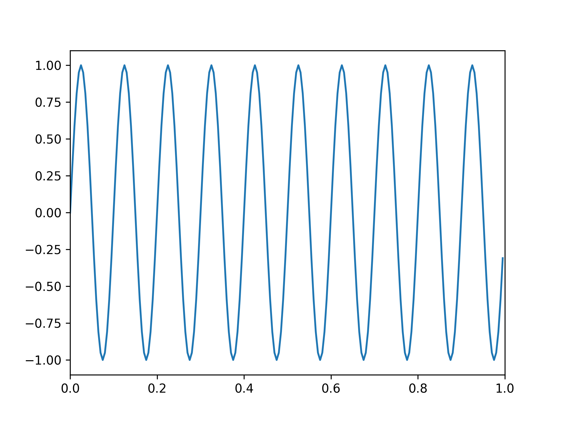
Generate a sinusoid:

import numpy as np
f1, f2, fs = 8, 10, 200  # Hz
t = np.linspace(0, 1, fs, endpoint=False)
x = np.sin(2*np.pi*t*f2)
import matplotlib.pyplot as plt

✓

plt.plot(t, x)
plt.axis([0, 1, -1.1, 1.1])

✗

plt.show()

✓

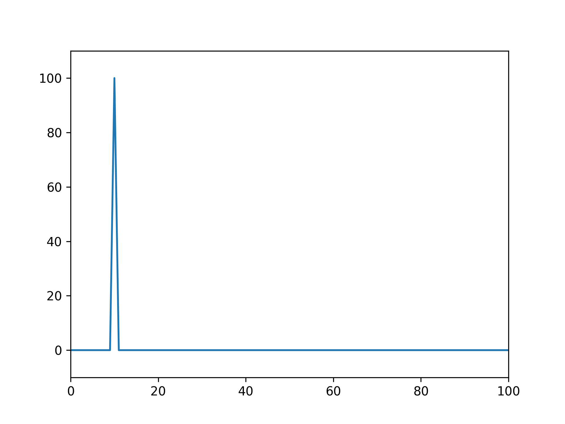
Its discrete Fourier transform has all of its energy in a single frequency bin:

from scipy.fft import rfft, rfftfreq
from scipy.signal import czt, czt_points

✓

plt.plot(rfftfreq(fs, 1/fs), abs(rfft(x)))

✗

plt.margins(0, 0.1)
plt.show()

✓

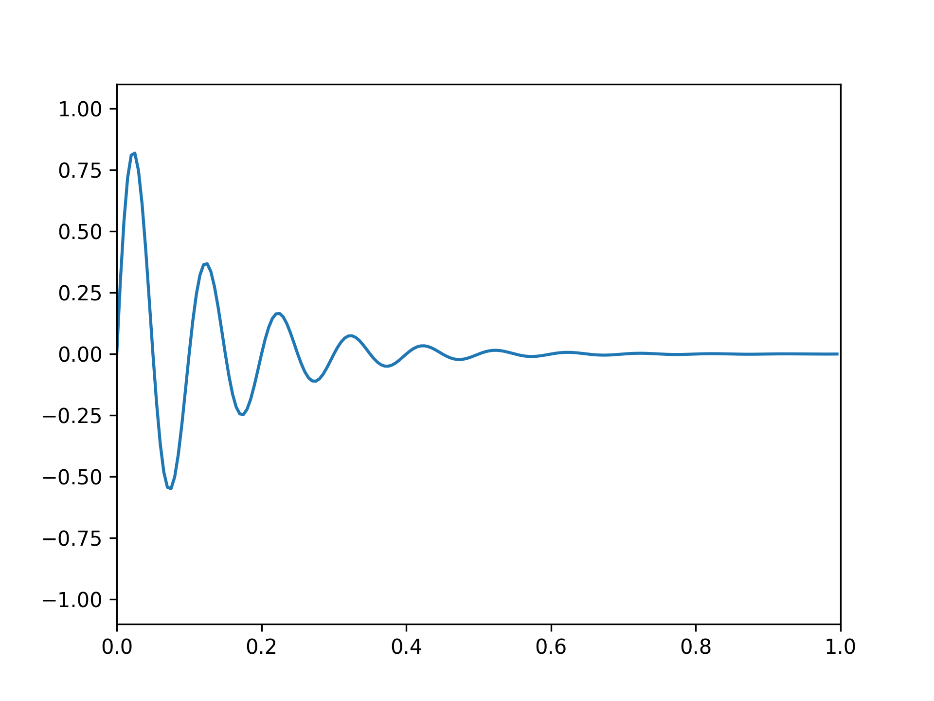
However, if the sinusoid is logarithmically-decaying:

x = np.exp(-t*f1) * np.sin(2*np.pi*t*f2)

✓

plt.plot(t, x)
plt.axis([0, 1, -1.1, 1.1])

✗

plt.show()

✓

the DFT will have spectral leakage:

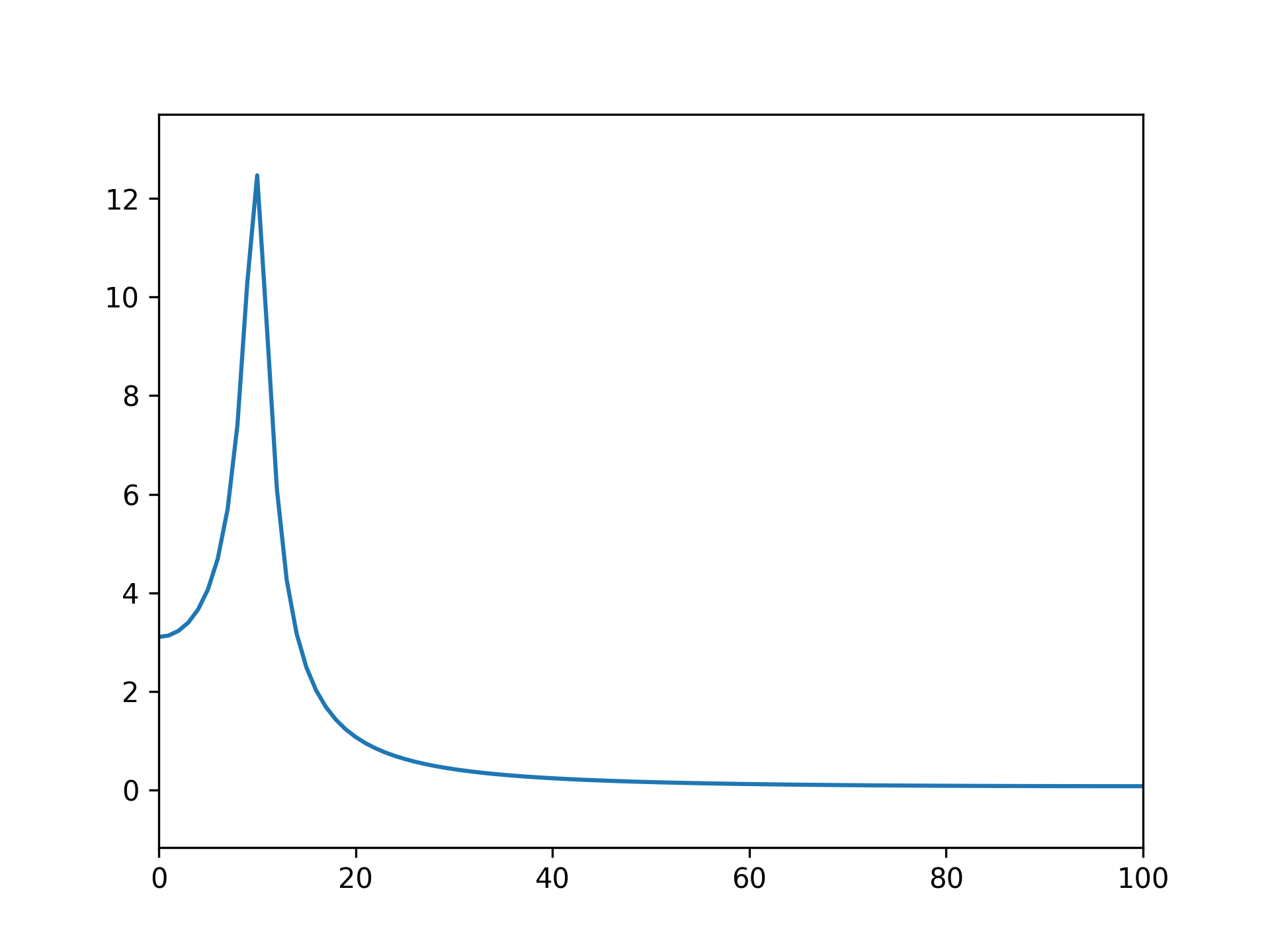
plt.plot(rfftfreq(fs, 1/fs), abs(rfft(x)))

✗

plt.margins(0, 0.1)
plt.show()

✓

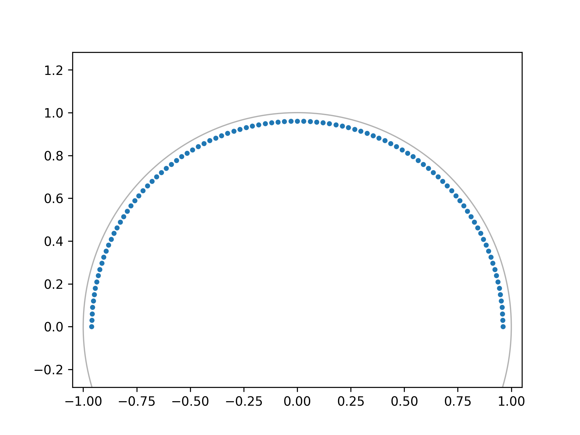
While the DFT always samples the z-transform around the unit circle, the chirp z-transform allows us to sample the Z-transform along any logarithmic spiral, such as a circle with radius smaller than unity:

M = fs // 2  # Just positive frequencies, like rfft
a = np.exp(-f1/fs)  # Starting point of the circle, radius < 1
w = np.exp(-1j*np.pi/M)  # "Step size" of circle
points = czt_points(M + 1, w, a)  # M + 1 to include Nyquist

✓

plt.plot(points.real, points.imag, '.')
plt.gca().add_patch(plt.Circle((0,0), radius=1, fill=False, alpha=.3))
plt.axis('equal'); plt.axis([-1.05, 1.05, -0.05, 1.05])

✗

plt.show()

✓

With the correct radius, this transforms the decaying sinusoid (and others with the same decay rate) without spectral leakage:

z_vals = czt(x, M + 1, w, a)  # Include Nyquist for comparison to rfft
freqs = np.angle(points)*fs/(2*np.pi)  # angle = omega, radius = sigma

✓

plt.plot(freqs, abs(z_vals))

✗

plt.margins(0, 0.1)
plt.show()

✓

Aliases

scipy.signal.czt