bundles / scipy latest / scipy / signal / _short_time_fft / ShortTimeFFT / extent
function
scipy.signal._short_time_fft:ShortTimeFFT.extent
Signature
def extent ( self , n : int , axes_seq : Literal['tf', 'ft'] = tf , center_bins : bool = False ) → tuple[float, float, float, float] Summary
Return minimum and maximum values time-frequency values.
Extended Summary
A tuple with four floats (t0, t1, f0, f1) for 'tf' and (f0, f1, t0, t1) for 'ft' is returned describing the corners of the time-frequency domain of the ~ShortTimeFFT.stft. That tuple can be passed to matplotlib.pyplot.imshow as a parameter with the same name.
Parameters
n: intNumber of samples in input signal.
axes_seq: {'tf', 'ft'}Return time extent first and then frequency extent or vice versa.
center_bins: boolIf set (default
False), the values of the time slots and frequency bins are moved from the side the middle. This is useful, when plotting the~ShortTimeFFT.stftvalues as step functions, i.e., with no interpolation.
Examples
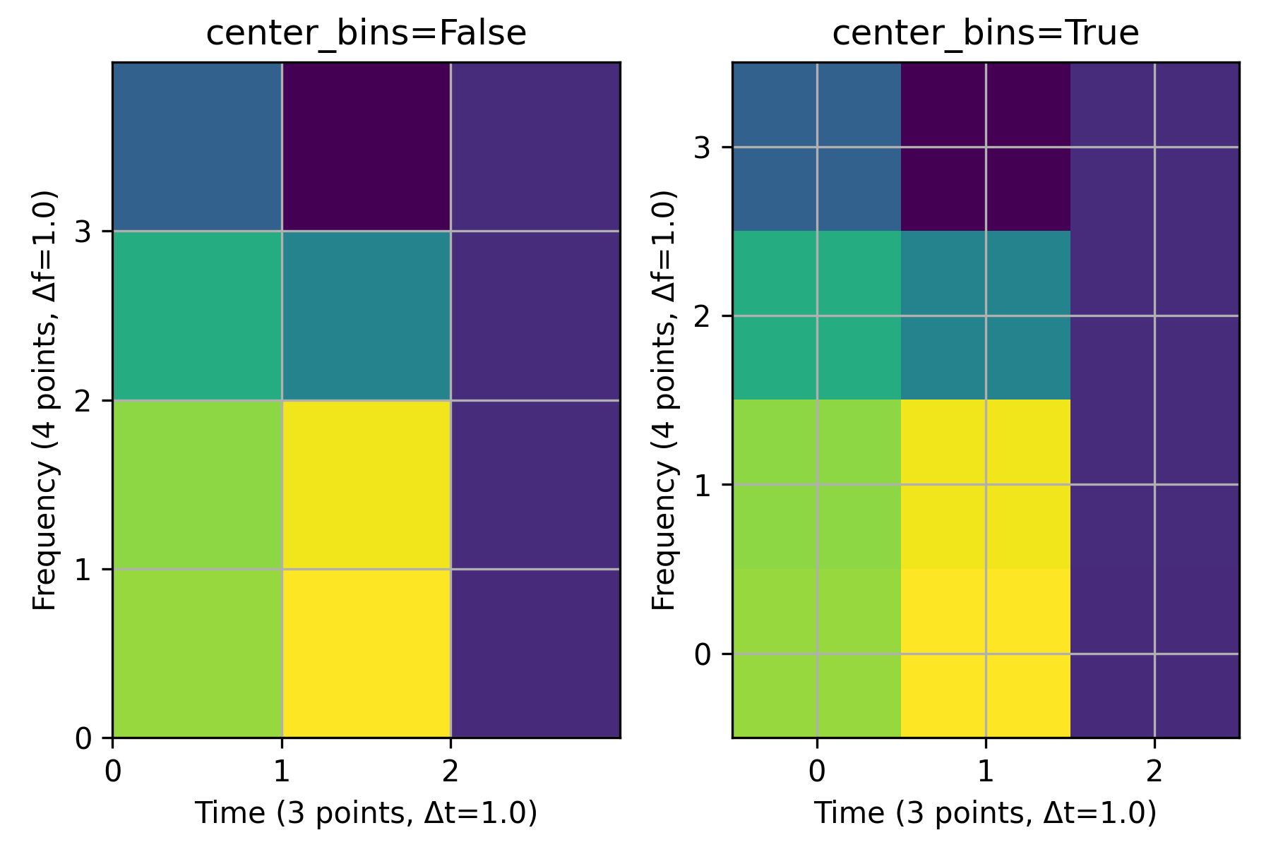
The following two plots illustrate the effect of the parameter `center_bins`: The grid lines represent the three time and the four frequency values of the STFT. The left plot, where ``(t0, t1, f0, f1) = (0, 3, 0, 4)`` is passed as parameter ``extent`` to `~matplotlib.pyplot.imshow`, shows the standard behavior of the time and frequency values being at the lower edge of the corrsponding bin. The right plot, with ``(t0, t1, f0, f1) = (-0.5, 2.5, -0.5, 3.5)``, shows that the bins are centered over the respective values when passing ``center_bins=True``.import matplotlib.pyplot as plt import numpy as np from scipy.signal import ShortTimeFFT n, m = 12, 6 SFT = ShortTimeFFT.from_window('hann', fs=m, nperseg=m, noverlap=0) Sxx = SFT.stft(np.cos(np.arange(n))) # produces a colorful plot fig, axx = plt.subplots(1, 2, tight_layout=True, figsize=(6., 4.))✓
for ax_, center_bins in zip(axx, (False, True)):
    ax_.imshow(abs(Sxx), origin='lower', interpolation=None, aspect='equal',
               cmap='viridis', extent=SFT.extent(n, 'tf', center_bins))
    ax_.set_title(f"{center_bins=}")
    ax_.set_xlabel(f"Time ({SFT.p_num(n)} points, Δt={SFT.delta_t})")
    ax_.set_ylabel(f"Frequency ({SFT.f_pts} points, Δf={SFT.delta_f})")
    ax_.set_xticks(SFT.t(n))  # vertical grid line are timestamps
    ax_.set_yticks(SFT.f)  # horizontal grid line are frequency values
    ax_.grid(True)
✗
plt.show()
✓
See also
- matplotlib.pyplot.imshow
Display data as an image.
- scipy.signal.ShortTimeFFT
Class this method belongs to.
Aliases
-
scipy.signal.ShortTimeFFT.extent