bundles / scipy latest / scipy / interpolate / _fitpack2 / BivariateSpline / ev
function
scipy.interpolate._fitpack2:BivariateSpline.ev
Signature
def ev ( self , xi , yi , dx = 0 , dy = 0 ) Summary
Evaluate the spline at points
Extended Summary
Returns the interpolated value at (xi[i], yi[i]), i=0,...,len(xi)-1.
Parameters
xi, yi: array_likeInput coordinates. Standard Numpy broadcasting is obeyed. The ordering of axes is consistent with
np.meshgrid(..., indexing="ij")and inconsistent with the default orderingnp.meshgrid(..., indexing="xy").dx: int, optionalOrder of x-derivative
dy: int, optionalOrder of y-derivative
Examples
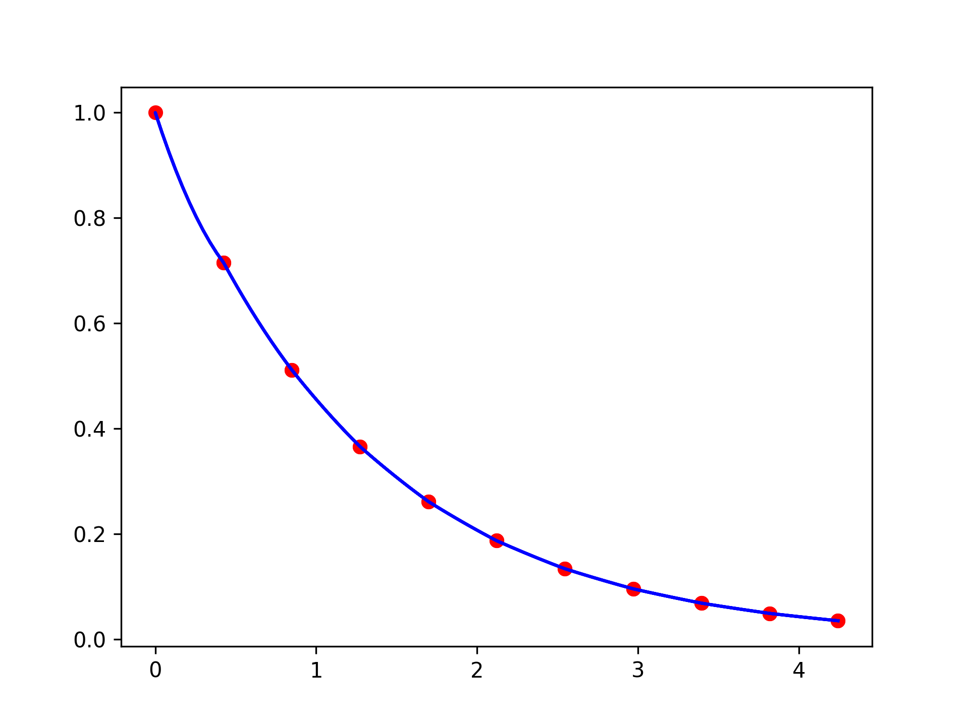
Suppose that we want to bilinearly interpolate an exponentially decaying function in 2 dimensions.import numpy as np from scipy.interpolate import RectBivariateSpline def f(x, y): return np.exp(-np.sqrt((x / 2) ** 2 + y**2))✓
xarr = np.linspace(-3, 3, 21)
yarr = np.linspace(-3, 3, 21)
xgrid, ygrid = np.meshgrid(xarr, yarr, indexing="ij")
zdata = f(xgrid, ygrid)
rbs = RectBivariateSpline(xarr, yarr, zdata, kx=1, ky=1)
✓
xinterp = np.linspace(-3, 3, 201)
yinterp = np.linspace(3, -3, 201)
zinterp = rbs.ev(xinterp, yinterp)
✓
import matplotlib.pyplot as plt
fig = plt.figure()
ax1 = fig.add_subplot(1, 1, 1)
✓
ax1.plot(np.sqrt(xarr**2 + yarr**2), np.diag(zdata), "or")
ax1.plot(np.sqrt(xinterp**2 + yinterp**2), zinterp, "-b")
✗
plt.show()
✓
Aliases
-
scipy.interpolate.BivariateSpline.ev