`scipy.stats._distribution_infrastructure:UnivariateDistribution.plot`

Signature

   def     plot (    self    ,    x    =  x   ,    y    =  None   ,  * ,     t    =  None   ,    ax    =  None     )

Plot a function of the distribution.

Convenience function for quick visualization of the distribution underlying the random variable.

x, y : str, optional: String indicating the quantities to be used as the abscissa and ordinate (horizontal and vertical coordinates), respectively. Defaults are 'x' (the domain of the random variable) and either 'pdf' (the probability density function) (continuous) or 'pdf' (the probability density function) (discrete). Valid values are: 'x', 'pdf', 'pmf', 'cdf', 'ccdf', 'icdf', 'iccdf', 'logpdf', 'logpmf', 'logcdf', 'logccdf', 'ilogcdf', 'ilogccdf'.
t : 3-tuple of (str, float, float), optional: Tuple indicating the limits within which the quantities are plotted. The default is ('cdf', 0.0005, 0.9995) if the domain is infinite, indicating that the central 99.9% of the distribution is to be shown; otherwise, endpoints of the support are used where they are finite. Valid values are: 'x', 'cdf', 'ccdf', 'icdf', 'iccdf', 'logcdf', 'logccdf', 'ilogcdf', 'ilogccdf'.
ax : `matplotlib.axes`, optional: Axes on which to generate the plot. If not provided, use the current axes.

ax : `matplotlib.axes`: Axes on which the plot was generated. The plot can be customized by manipulating this object.

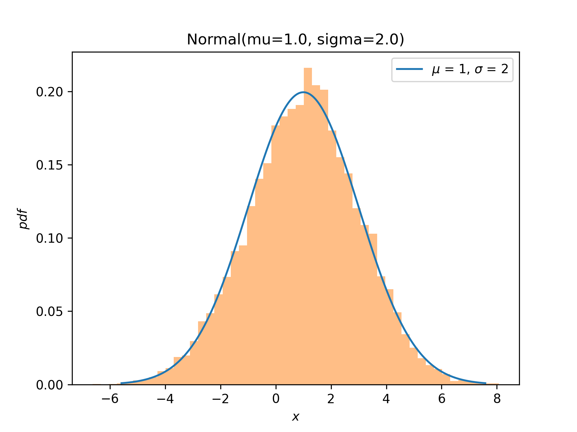
Instantiate a distribution with the desired parameters:

import numpy as np
import matplotlib.pyplot as plt
from scipy import stats
X = stats.Normal(mu=1., sigma=2.)

✓

Plot the PDF over the central 99.9% of the distribution. Compare against a histogram of a random sample.

ax = X.plot()
sample = X.sample(10000)

✓

ax.hist(sample, density=True, bins=50, alpha=0.5)

✗

plt.show()

✓

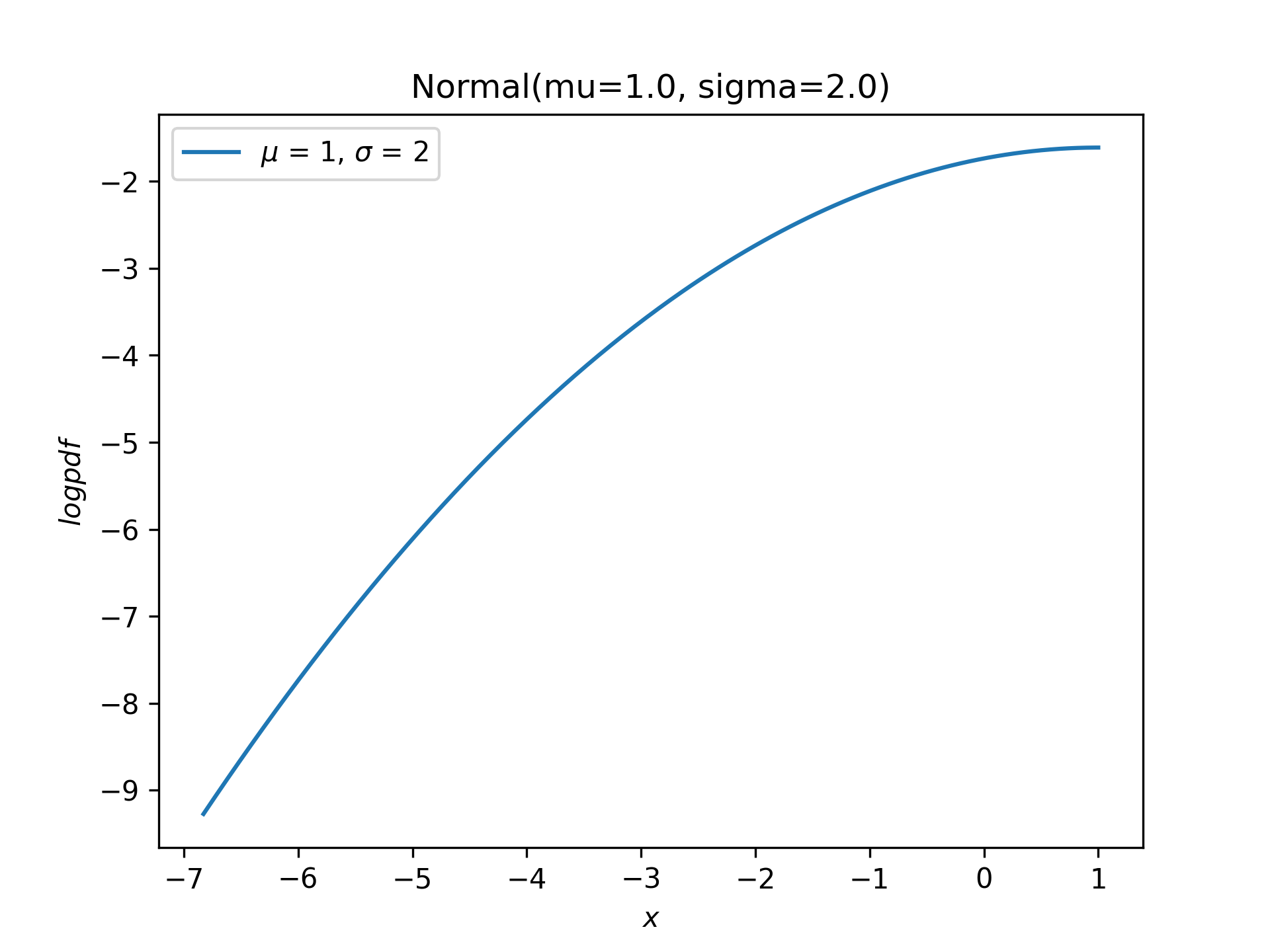
Plot ``logpdf(x)`` as a function of ``x`` in the left tail, where the log of the CDF is between -10 and ``np.log(0.5)``.

X.plot('x', 'logpdf', t=('logcdf', -10, np.log(0.5)))

✗

plt.show()

✓

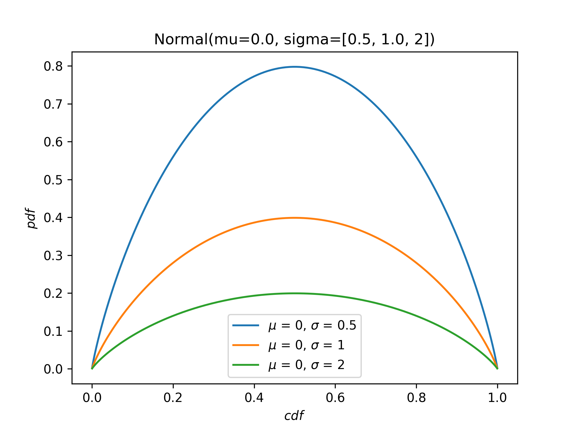
Plot the PDF of the normal distribution as a function of the CDF for various values of the scale parameter.

X = stats.Normal(mu=0., sigma=[0.5, 1., 2])

✓

X.plot('cdf', 'pdf')

✗

plt.show()

✓