`numpy.random._generator:Generator.multivariate_normal`

Signature

   def     multivariate_normal (    mean    ,    cov    ,    size    =  None   ,    check_valid    =  warn   ,    tol    =  1e-08   ,  * ,     method    =  svd     )

Summary

Draw random samples from a multivariate normal distribution.

Extended Summary

The multivariate normal, multinormal or Gaussian distribution is a generalization of the one-dimensional normal distribution to higher dimensions. Such a distribution is specified by its mean and covariance matrix. These parameters are analogous to the mean (average or "center") and variance (the squared standard deviation, or "width") of the one-dimensional normal distribution.

Parameters

mean : 1-D array_like, of length N: Mean of the N-dimensional distribution.
cov : 2-D array_like, of shape (N, N): Covariance matrix of the distribution. It must be symmetric and positive-semidefinite for proper sampling.
size : int or tuple of ints, optional: Given a shape of, for example, (m,n,k), m*n*k samples are generated, and packed in an m-by-n-by-k arrangement. Because each sample is N-dimensional, the output shape is (m,n,k,N). If no shape is specified, a single (N-D) sample is returned.
check_valid : { 'warn', 'raise', 'ignore' }, optional: Behavior when the covariance matrix is not positive semidefinite.
tol : float, optional: Tolerance when checking the singular values in covariance matrix. cov is cast to double before the check.
method : { 'svd', 'eigh', 'cholesky'}, optional: The cov input is used to compute a factor matrix A such that A @ A.T = cov. This argument is used to select the method used to compute the factor matrix A. The default method 'svd' is the slowest, while 'cholesky' is the fastest but less robust than the slowest method. The method eigh uses eigen decomposition to compute A and is faster than svd but slower than cholesky.

Returns

out : ndarray

The drawn samples, of shape size, if that was provided. If not, the shape is (N,).

In other words, each entry out[i,j,...,:] is an N-dimensional value drawn from the distribution.

Notes

The mean is a coordinate in N-dimensional space, which represents the location where samples are most likely to be generated. This is analogous to the peak of the bell curve for the one-dimensional or univariate normal distribution.

Covariance indicates the level to which two variables vary together. From the multivariate normal distribution, we draw N-dimensional samples, $X = [x_{1}, x_{2}, ..., x_{N}]$ . The covariance matrix element $C_{ij}$ is the covariance of $x_{i}$ and $x_{j}$ . The element $C_{ii}$ is the variance of $x_{i}$ (i.e. its "spread").

Instead of specifying the full covariance matrix, popular approximations include:

Spherical covariance (cov is a multiple of the identity matrix)
Diagonal covariance (cov has non-negative elements, and only on the diagonal)

This geometrical property can be seen in two dimensions by plotting generated data-points:

>>> mean = [0, 0]
>>> cov = [[1, 0], [0, 100]]  # diagonal covariance

Diagonal covariance means that the variables are independent, and the probability density contours have their axes aligned with the coordinate axes:

>>> import matplotlib.pyplot as plt
>>> rng = np.random.default_rng()
>>> x, y = rng.multivariate_normal(mean, cov, 5000).T
>>> plt.plot(x, y, 'x')
>>> plt.axis('equal')
>>> plt.show()

Note that the covariance matrix must be positive semidefinite (a.k.a. nonnegative-definite). Otherwise, the behavior of this method is undefined and backwards compatibility is not guaranteed.

This function internally uses linear algebra routines, and thus results may not be identical (even up to precision) across architectures, OSes, or even builds. For example, this is likely if cov has multiple equal singular values and method is 'svd' (default). In this case, method='cholesky' may be more robust.

Examples

mean = (1, 2)
cov = [[1, 0], [0, 1]]
rng = np.random.default_rng()
x = rng.multivariate_normal(mean, cov, (3, 3))
x.shape

✓

We can use a different method other than the default to factorize cov:

y = rng.multivariate_normal(mean, cov, (3, 3), method='cholesky')
y.shape

✓

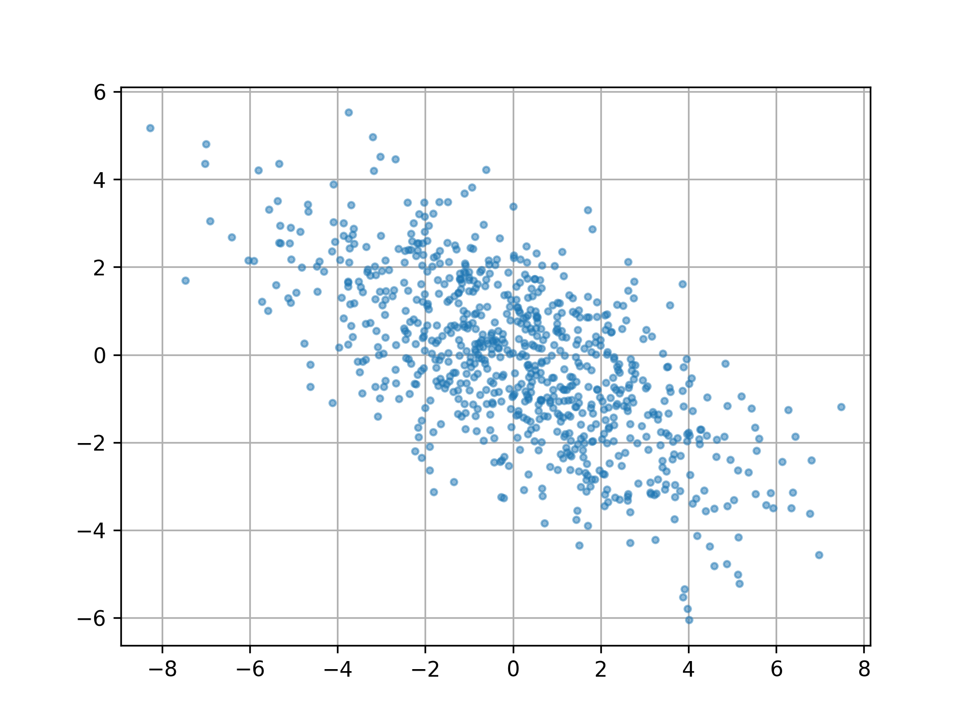
Here we generate 800 samples from the bivariate normal distribution with mean [0, 0] and covariance matrix [[6, -3], [-3, 3.5]]. The expected variances of the first and second components of the sample are 6 and 3.5, respectively, and the expected correlation coefficient is -3/sqrt(6*3.5) ≈ -0.65465.

cov = np.array([[6, -3], [-3, 3.5]])
pts = rng.multivariate_normal([0, 0], cov, size=800)

✓

Check that the mean, covariance, and correlation coefficient of the sample are close to the expected values:

pts.mean(axis=0)
np.cov(pts.T)
np.corrcoef(pts.T)[0, 1]

✗

We can visualize this data with a scatter plot. The orientation of the point cloud illustrates the negative correlation of the components of this sample.

import matplotlib.pyplot as plt

✓

plt.plot(pts[:, 0], pts[:, 1], '.', alpha=0.5)
plt.axis('equal')

✗

plt.grid()
plt.show()

✓

Aliases

numpy.random.Generator.multivariate_normal