bundles / scipy latest / scipy / signal / _spectral_py / lombscargle

function

`scipy.signal._spectral_py:lombscargle`

source: /scipy/signal/_spectral_py.py :19

Signature

   def     lombscargle (    x  :  npt.ArrayLike    ,    y  :  npt.ArrayLike    ,    freqs  :  npt.ArrayLike    ,  * ,     precenter  :  bool    =  <object object at 0x0000>   ,    normalize  :  bool | Literal['power', 'normalize', 'amplitude']    =  False   ,    weights  :  npt.NDArray | None    =  None   ,    floating_mean  :  bool    =  False     )   →  npt.NDArray

Summary

Compute the generalized Lomb-Scargle periodogram.

Extended Summary

The Lomb-Scargle periodogram was developed by Lomb ^[1] and further extended by Scargle ^[2] to find, and test the significance of weak periodic signals with uneven temporal sampling. The algorithm used here is based on a weighted least-squares fit of the form y(ω) = a*cos(ω*x) + b*sin(ω*x) + c, where the fit is calculated for each frequency independently. This algorithm was developed by Zechmeister and Kürster which improves the Lomb-Scargle periodogram by enabling the weighting of individual samples and calculating an unknown y offset (also called a "floating-mean" model) ^[3]. For more details, and practical considerations, see the excellent reference on the Lomb-Scargle periodogram ^[4].

When normalize is False (or "power") (default) the computed periodogram is unnormalized, it takes the value (A**2) * N/4 for a harmonic signal with amplitude A for sufficiently large N. Where N is the length of x or y.

When normalize is True (or "normalize") the computed periodogram is normalized by the residuals of the data around a constant reference model (at zero).

When normalize is "amplitude" the computed periodogram is the complex representation of the amplitude and phase.

Input arrays should be 1-D of a real floating data type, which are converted into float64 arrays before processing.

Parameters

x : array_like: Sample times.
y : array_like: Measurement values. Values are assumed to have a baseline of y = 0. If there is a possibility of a y offset, it is recommended to set floating_mean to True.
freqs : array_like: Angular frequencies (e.g., having unit rad/s=2π/s for x having unit s) for output periodogram. Frequencies are normally >= 0, as any peak at -freq will also exist at +freq.
precenter : bool, optional: Pre-center measurement values by subtracting the mean, if True. This is a legacy parameter and unnecessary if floating_mean is True.
deprecated 1.17.0
The precenter argument is deprecated and will be removed in SciPy 1.19.0. The functionality can be substituted by passing y - y.mean() to y.
normalize : bool | str, optional: Compute normalized or complex (amplitude + phase) periodogram. Valid options are: False/"power", True/"normalize", or "amplitude".
weights : array_like, optional: Weights for each sample. Weights must be nonnegative.
floating_mean : bool, optional: Determines a y offset for each frequency independently, if True. Else the y offset is assumed to be 0.

Returns

pgram : array_like: Lomb-Scargle periodogram.

Raises

: ValueError: If any of the input arrays x, y, freqs, or weights are not 1D, or if any are zero length. Or, if the input arrays x, y, and weights do not have the same shape as each other.
: ValueError: If any weight is < 0, or the sum of the weights is <= 0.
: ValueError: If the normalize parameter is not one of the allowed options.

Notes

The algorithm used will not automatically account for any unknown y offset, unless floating_mean is True. Therefore, for most use cases, if there is a possibility of a y offset, it is recommended to set floating_mean to True. Furthermore, floating_mean accounts for sample weights, and will also correct for any bias due to consistently missing observations at peaks and/or troughs.

The legacy concept of "pre-centering" entails removing the mean from parameter y before processing, i.e., passing y - y.mean() instead of setting the parameter floating_mean to True.

When the normalize parameter is "amplitude", for any frequency in freqs that is below (2*pi)/(x.max() - x.min()), the predicted amplitude will tend towards infinity. The concept of a "Nyquist frequency" limit (see Nyquist-Shannon sampling theorem) is not generally applicable to unevenly sampled data. Therefore, with unevenly sampled data, valid frequencies in freqs can often be much higher than expected for those familiar with methods like FFT.

Array API Standard Support

lombscargle has experimental support for Python Array API Standard compatible backends in addition to NumPy. Please consider testing these features by setting an environment variable SCIPY_ARRAY_API=1 and providing CuPy, PyTorch, JAX, or Dask arrays as array arguments. The following combinations of backend and device (or other capability) are supported.

====================  ====================  ====================
Library               CPU                   GPU
====================  ====================  ====================
NumPy                 ✅                     n/a                 
CuPy                  n/a                   ⛔                   
PyTorch               ⛔                     ⛔                   
JAX                   ⛔                     ⛔                   
Dask                  ⛔                     n/a                 
====================  ====================  ====================

See dev-arrayapi for more information.

Examples

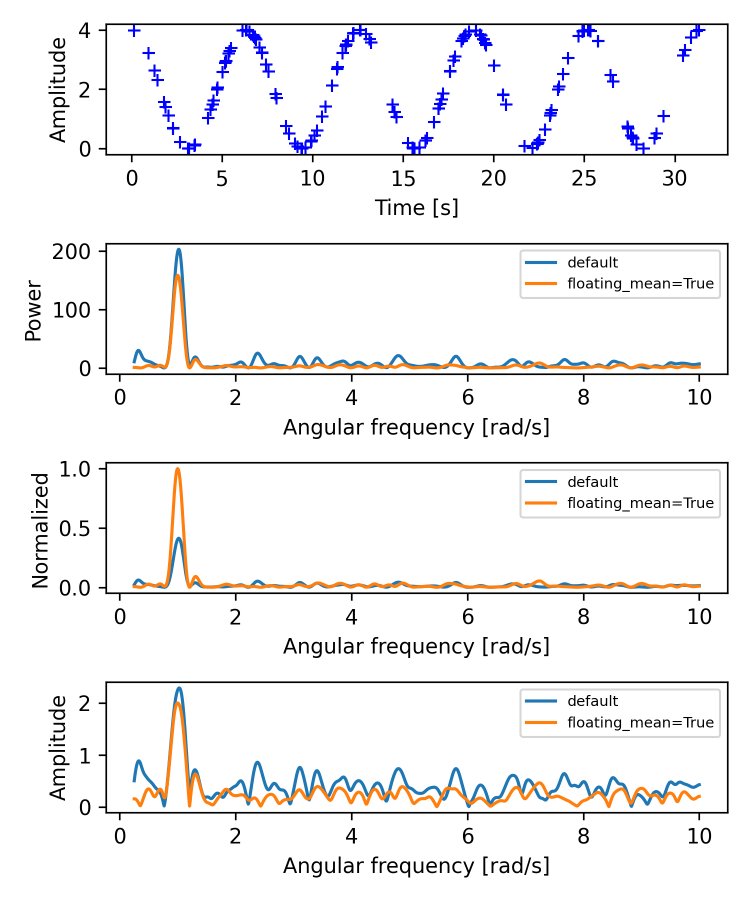
import numpy as np
rng = np.random.default_rng()

✓

First define some input parameters for the signal:

A = 2.  # amplitude
c = 2.  # offset
w0 = 1.  # rad/sec
nin = 150
nout = 1002

✓

Randomly generate sample times:

x = rng.uniform(0, 10*np.pi, nin)

✓

Plot a sine wave for the selected times:

y = A * np.cos(w0*x) + c

✓

Define the array of frequencies for which to compute the periodogram:

w = np.linspace(0.25, 10, nout)

✓

Calculate Lomb-Scargle periodogram for each of the normalize options:

from scipy.signal import lombscargle
pgram_power = lombscargle(x, y, w, normalize=False)
pgram_norm = lombscargle(x, y, w, normalize=True)
pgram_amp = lombscargle(x, y, w, normalize='amplitude')
pgram_power_f = lombscargle(x, y, w, normalize=False, floating_mean=True)
pgram_norm_f = lombscargle(x, y, w, normalize=True, floating_mean=True)
pgram_amp_f = lombscargle(x, y, w, normalize='amplitude', floating_mean=True)

✓

Now make a plot of the input data:

import matplotlib.pyplot as plt
fig, (ax_t, ax_p, ax_n, ax_a) = plt.subplots(4, 1, figsize=(5, 6))

✓

ax_t.plot(x, y, 'b+')
ax_t.set_xlabel('Time [s]')
ax_t.set_ylabel('Amplitude')

✗

Then plot the periodogram for each of the normalize options, as well as with and without floating_mean=True:

ax_p.plot(w, pgram_power, label='default')
ax_p.plot(w, pgram_power_f, label='floating_mean=True')
ax_p.set_xlabel('Angular frequency [rad/s]')
ax_p.set_ylabel('Power')
ax_p.legend(prop={'size': 7})
ax_n.plot(w, pgram_norm, label='default')
ax_n.plot(w, pgram_norm_f, label='floating_mean=True')
ax_n.set_xlabel('Angular frequency [rad/s]')
ax_n.set_ylabel('Normalized')
ax_n.legend(prop={'size': 7})
ax_a.plot(w, np.abs(pgram_amp), label='default')
ax_a.plot(w, np.abs(pgram_amp_f), label='floating_mean=True')
ax_a.set_xlabel('Angular frequency [rad/s]')
ax_a.set_ylabel('Amplitude')
ax_a.legend(prop={'size': 7})

✗

plt.tight_layout()
plt.show()

✓

Aliases

scipy.signal.lombscargle

`scipy.signal._spectral_py:lombscargle`

Signature

Summary

Extended Summary

Parameters

Returns

Raises

Notes

Examples

See also

Aliases

Referenced by

This package