`scipy.signal._spectral_py:csd`

source: /scipy/signal/_spectral_py.py :690

Signature

   def     csd (    x    ,    y    ,    fs    =  1.0   ,    window    =  hann_periodic   ,    nperseg    =  None   ,    noverlap    =  None   ,    nfft    =  None   ,    detrend    =  constant   ,    return_onesided    =  True   ,    scaling    =  density   ,    axis    =  -1   ,    average    =  mean     )

Summary

Estimate the cross power spectral density, Pxy, using Welch's method.

Parameters

x : array_like: Time series of measurement values
y : array_like: Time series of measurement values
fs : float, optional: Sampling frequency of the x and y time series. Defaults to 1.0.
window : str or tuple or array_like, optional: Desired window to use. If window is a string or tuple, it is passed to get_window to generate the window values, which are DFT-even by default. See get_window for a list of windows and required parameters. If window is array_like it will be used directly as the window and its length must be nperseg. Defaults to a periodic Hann window.
nperseg : int, optional: Length of each segment. Defaults to None, but if window is str or tuple, is set to 256, and if window is array_like, is set to the length of the window.
noverlap: int, optional: Number of points to overlap between segments. If None, noverlap = nperseg // 2. Defaults to None and may not be greater than nperseg.
nfft : int, optional: Length of the FFT used, if a zero padded FFT is desired. If None, the FFT length is nperseg. Defaults to None.
detrend : str or function or `False`, optional: Specifies how to detrend each segment. If detrend is a string, it is passed as the type argument to the detrend function. If it is a function, it takes a segment and returns a detrended segment. If detrend is False, no detrending is done. Defaults to 'constant'.
return_onesided : bool, optional: If True, return a one-sided spectrum for real data. If False return a two-sided spectrum. Defaults to True, but for complex data, a two-sided spectrum is always returned.
scaling : { 'density', 'spectrum' }, optional: Selects between computing the cross spectral density ('density') where Pxy has units of V**2/Hz and computing the cross spectrum ('spectrum') where Pxy has units of V**2, if x and y are measured in V and fs is measured in Hz. Defaults to 'density'
axis : int, optional: Axis along which the CSD is computed for both inputs; the default is over the last axis (i.e. axis=-1).
average : { 'mean', 'median' }, optional: Method to use when averaging periodograms. If the spectrum is complex, the average is computed separately for the real and imaginary parts. Defaults to 'mean'.
versionadded 1.2.0

Returns

f : ndarray: Array of sample frequencies.
Pxy : ndarray: Cross spectral density or cross power spectrum of x,y.

Notes

By convention, Pxy is computed with the conjugate FFT of X multiplied by the FFT of Y.

If the input series differ in length, the shorter series will be zero-padded to match.

An appropriate amount of overlap will depend on the choice of window and on your requirements. For the default Hann window an overlap of 50% is a reasonable trade-off between accurately estimating the signal power, while not over counting any of the data. Narrower windows may require a larger overlap.

The ratio of the cross spectrum (scaling='spectrum') divided by the cross spectral density (scaling='density') is the constant factor of sum(abs(window)**2)*fs / abs(sum(window))**2. If return_onesided is True, the values of the negative frequencies are added to values of the corresponding positive ones.

Consult the tutorial_SpectralAnalysis section of the user_guide for a discussion of the scalings of a spectral density and an (amplitude) spectrum.

Welch's method may be interpreted as taking the average over the time slices of a (cross-) spectrogram. Internally, this function utilizes the ShortTimeFFT to determine the required (cross-) spectrogram. An example below illustrates that it is straightforward to calculate Pxy directly with the ShortTimeFFT. However, there are some notable differences in the behavior of the ShortTimeFFT:

There is no direct ShortTimeFFT equivalent for the csd parameter combination return_onesided=True, scaling='density', since fft_mode='onesided2X' requires 'psd' scaling. The is due to csd returning the doubled squared magnitude in this case, which does not have a sensible interpretation.
ShortTimeFFT uses float64 / complex128 internally, which is due to the behavior of the utilized fft module. Thus, those are the dtypes being returned. The csd function casts the return values to float32 / complex64 if the input is float32 / complex64 as well.
The csd function calculates np.conj(Sx[q,p]) * Sy[q,p], whereas ~ShortTimeFFT.spectrogram calculates Sx[q,p] * np.conj(Sy[q,p]) where Sx[q,p], Sy[q,p] are the STFTs of x and y. Also, the window positioning is different.

Array API Standard Support

csd has experimental support for Python Array API Standard compatible backends in addition to NumPy. Please consider testing these features by setting an environment variable SCIPY_ARRAY_API=1 and providing CuPy, PyTorch, JAX, or Dask arrays as array arguments. The following combinations of backend and device (or other capability) are supported.

====================  ====================  ====================
Library               CPU                   GPU
====================  ====================  ====================
NumPy                 ✅                     n/a                 
CuPy                  n/a                   ⛔                   
PyTorch               ⛔                     ⛔                   
JAX                   ⛔                     ⛔                   
Dask                  ⛔                     n/a                 
====================  ====================  ====================

See dev-arrayapi for more information.

Examples

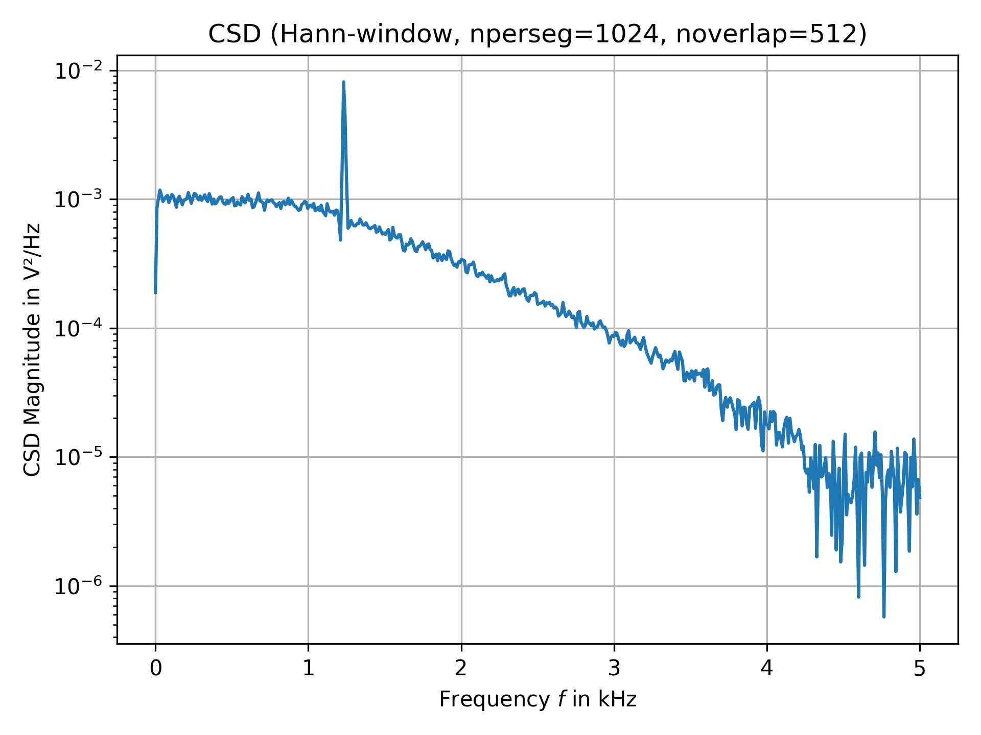
The following example plots the cross power spectral density of two signals with some common features:

import numpy as np
from scipy import signal
import matplotlib.pyplot as plt
rng = np.random.default_rng()

# Generate two test signals with some common features:
N, fs = 100_000, 10e3  # number of samples and sampling frequency
amp, freq = 20, 1234.0  # amplitude and frequency of utilized sine signal
noise_power = 0.001 * fs / 2
time = np.arange(N) / fs
b, a = signal.butter(2, 0.25, 'low')
x = rng.normal(scale=np.sqrt(noise_power), size=time.shape)
y = signal.lfilter(b, a, x)
x += amp*np.sin(2*np.pi*freq*time)
y += rng.normal(scale=0.1*np.sqrt(noise_power), size=time.shape)

# Compute and plot the magnitude of the cross spectral density:
nperseg, noverlap, win = 1024, 512, 'hann'
f, Pxy = signal.csd(x, y, fs, win, nperseg, noverlap)
fig0, ax0 = plt.subplots(tight_layout=True)

✓

ax0.set_title(f"CSD ({win.title()}-window, {nperseg=}, {noverlap=})")
ax0.set(xlabel="Frequency $f$ in kHz", ylabel="CSD Magnitude in V²/Hz")
ax0.semilogy(f/1e3, np.abs(Pxy))

✗

ax0.grid()
plt.show()

✓

The cross spectral density is calculated by taking the average over the time slices of a spectrogram:

SFT = signal.ShortTimeFFT.from_window('hann', fs, nperseg, noverlap,
                                      scale_to='psd', fft_mode='onesided2X',
                                      phase_shift=None)
Sxy1 = SFT.spectrogram(y, x, detr='constant', k_offset=nperseg//2,
                       p0=0, p1=(N-noverlap) // SFT.hop)
Pxy1 = Sxy1.mean(axis=-1)
np.allclose(Pxy, Pxy1)  # same result as with csd()

✓

As discussed in the Notes section, the results of using an approach analogous to the code snippet above and the `csd` function may deviate due to implementation details. Note that the code snippet above can be easily adapted to determine other statistical properties than the mean value.

`scipy.signal._spectral_py:csd`

Signature

Summary

Parameters

Returns

Notes

Examples

See also

Aliases

Referenced by

This package