bundles / scipy latest / scipy / signal / _spectral_py / welch

function

`scipy.signal._spectral_py:welch`

source: /scipy/signal/_spectral_py.py :515

Signature

   def     welch (    x    ,    fs    =  1.0   ,    window    =  hann_periodic   ,    nperseg    =  None   ,    noverlap    =  None   ,    nfft    =  None   ,    detrend    =  constant   ,    return_onesided    =  True   ,    scaling    =  density   ,    axis    =  -1   ,    average    =  mean     )

Summary

Estimate power spectral density using Welch's method.

Extended Summary

Welch's method ^[1] computes an estimate of the power spectral density by dividing the data into overlapping segments, computing a modified periodogram for each segment and averaging the periodograms.

Parameters

x : array_like: Time series of measurement values
fs : float, optional: Sampling frequency of the x time series. Defaults to 1.0.
window : str or tuple or array_like, optional: Desired window to use. If window is a string or tuple, it is passed to get_window to generate the window values, which are DFT-even by default. See get_window for a list of windows and required parameters. If window is array_like it will be used directly as the window and its length must be nperseg. Defaults to a periodic Hann window.
nperseg : int, optional: Length of each segment. Defaults to None, but if window is str or tuple, is set to 256, and if window is array_like, is set to the length of the window.
noverlap : int, optional: Number of points to overlap between segments. If None, noverlap = nperseg // 2. Defaults to None.
nfft : int, optional: Length of the FFT used, if a zero padded FFT is desired. If None, the FFT length is nperseg. Defaults to None.
detrend : str or function or `False`, optional: Specifies how to detrend each segment. If detrend is a string, it is passed as the type argument to the detrend function. If it is a function, it takes a segment and returns a detrended segment. If detrend is False, no detrending is done. Defaults to 'constant'.
return_onesided : bool, optional: If True, return a one-sided spectrum for real data. If False return a two-sided spectrum. Defaults to True, but for complex data, a two-sided spectrum is always returned.
scaling : { 'density', 'spectrum' }, optional: Selects between computing the power spectral density ('density') where Pxx has units of V**2/Hz and computing the squared magnitude spectrum ('spectrum') where Pxx has units of V**2, if x is measured in V and fs is measured in Hz. Defaults to 'density'
axis : int, optional: Axis along which the periodogram is computed; the default is over the last axis (i.e. axis=-1).
average : { 'mean', 'median' }, optional: Method to use when averaging periodograms. Defaults to 'mean'.
versionadded 1.2.0

Returns

f : ndarray: Array of sample frequencies.
Pxx : ndarray: Power spectral density or power spectrum of x.

Notes

An appropriate amount of overlap will depend on the choice of window and on your requirements. For the default Hann window an overlap of 50% is a reasonable trade-off between accurately estimating the signal power, while not over counting any of the data. Narrower windows may require a larger overlap. If noverlap is 0, this method is equivalent to Bartlett's method ^[2].

The ratio of the squared magnitude (scaling='spectrum') divided by the spectral power density (scaling='density') is the constant factor of sum(abs(window)**2)*fs / abs(sum(window))**2. If return_onesided is True, the values of the negative frequencies are added to values of the corresponding positive ones.

Consult the tutorial_SpectralAnalysis section of the user_guide for a discussion of the scalings of the power spectral density and the (squared) magnitude spectrum.

Array API Standard Support

welch has experimental support for Python Array API Standard compatible backends in addition to NumPy. Please consider testing these features by setting an environment variable SCIPY_ARRAY_API=1 and providing CuPy, PyTorch, JAX, or Dask arrays as array arguments. The following combinations of backend and device (or other capability) are supported.

====================  ====================  ====================
Library               CPU                   GPU
====================  ====================  ====================
NumPy                 ✅                     n/a                 
CuPy                  n/a                   ⛔                   
PyTorch               ⛔                     ⛔                   
JAX                   ⛔                     ⛔                   
Dask                  ⛔                     n/a                 
====================  ====================  ====================

See dev-arrayapi for more information.

Examples

import numpy as np
from scipy import signal
import matplotlib.pyplot as plt
rng = np.random.default_rng()

✓

Generate a test signal, a 2 Vrms sine wave at 1234 Hz, corrupted by 0.001 V**2/Hz of white noise sampled at 10 kHz.

fs = 10e3
N = 1e5
amp = 2*np.sqrt(2)
freq = 1234.0
noise_power = 0.001 * fs / 2
time = np.arange(N) / fs
x = amp*np.sin(2*np.pi*freq*time)
x += rng.normal(scale=np.sqrt(noise_power), size=time.shape)

✓

Compute and plot the power spectral density.

f, Pxx_den = signal.welch(x, fs, nperseg=1024)

✓

plt.semilogy(f, Pxx_den)
plt.ylim([0.5e-3, 1])
plt.xlabel('frequency [Hz]')
plt.ylabel('PSD [V**2/Hz]')

✗

plt.show()

✓

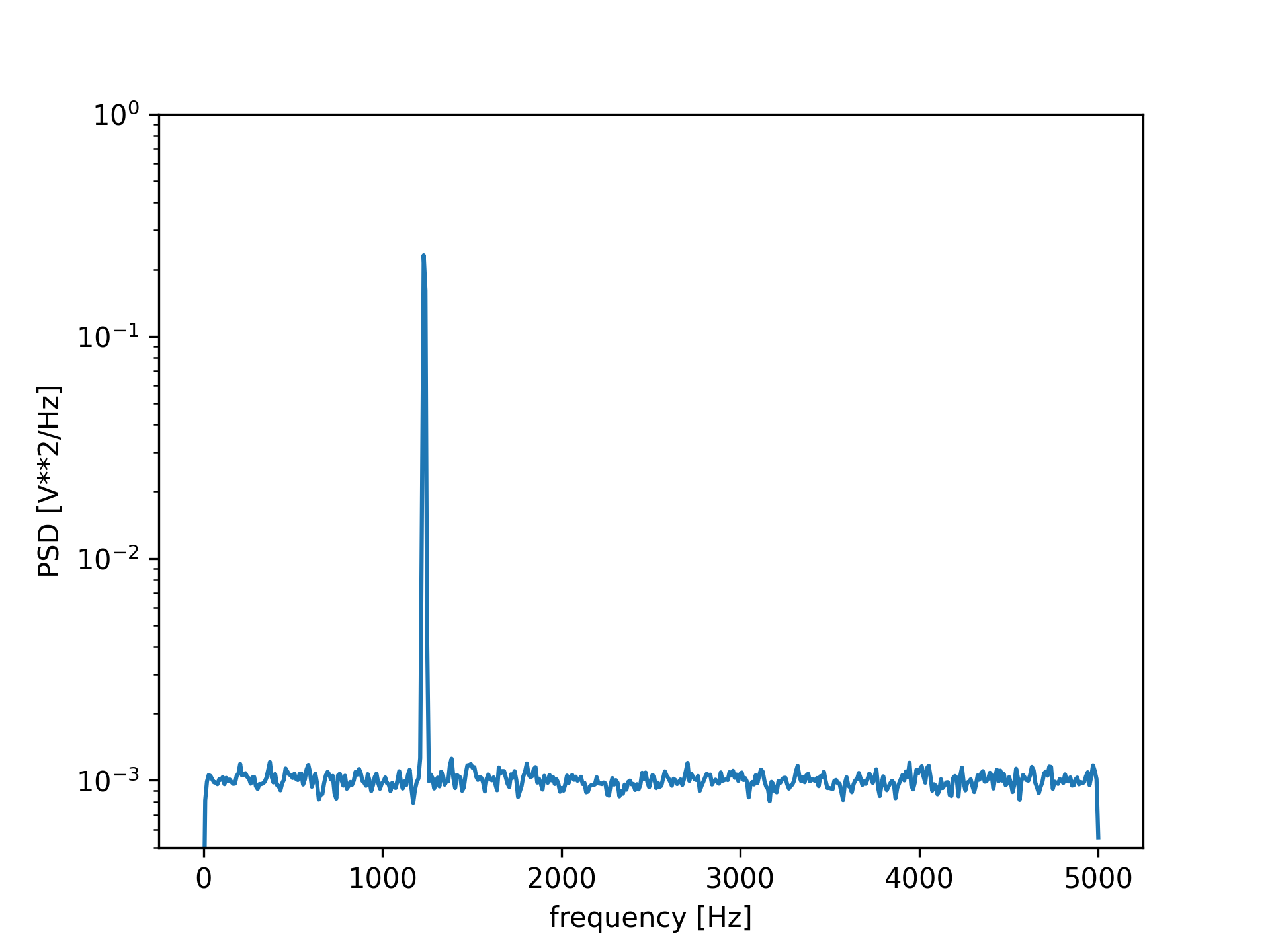
If we average the last half of the spectral density, to exclude the peak, we can recover the noise power on the signal.

np.mean(Pxx_den[256:])

✗

Now compute and plot the power spectrum.

f, Pxx_spec = signal.welch(x, fs, 'flattop', 1024, scaling='spectrum')

✓

plt.figure()
plt.semilogy(f, np.sqrt(Pxx_spec))
plt.xlabel('frequency [Hz]')
plt.ylabel('Linear spectrum [V RMS]')

✗

plt.show()

✓

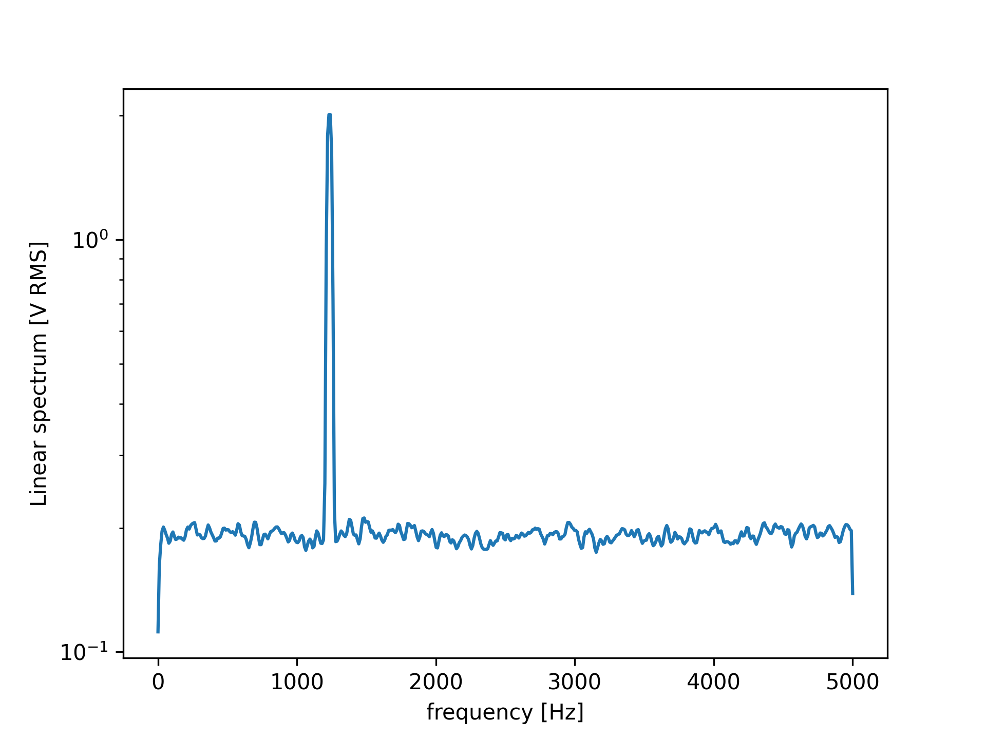
The peak height in the power spectrum is an estimate of the RMS amplitude.

np.sqrt(Pxx_spec.max())

✗

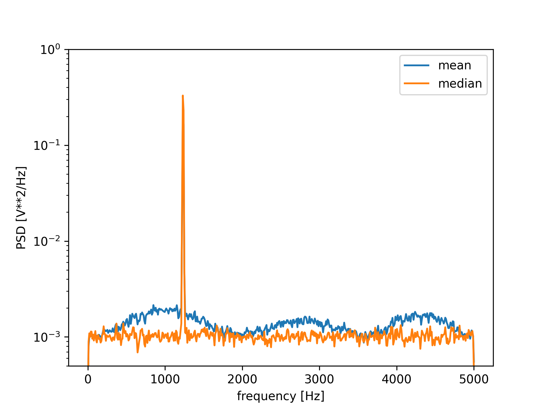
If we now introduce a discontinuity in the signal, by increasing the amplitude of a small portion of the signal by 50, we can see the corruption of the mean average power spectral density, but using a median average better estimates the normal behaviour.

x[int(N//2):int(N//2)+10] *= 50.
f, Pxx_den = signal.welch(x, fs, nperseg=1024)
f_med, Pxx_den_med = signal.welch(x, fs, nperseg=1024, average='median')

✓

plt.semilogy(f, Pxx_den, label='mean')
plt.semilogy(f_med, Pxx_den_med, label='median')
plt.ylim([0.5e-3, 1])
plt.xlabel('frequency [Hz]')
plt.ylabel('PSD [V**2/Hz]')
plt.legend()

✗

plt.show()

✓

`scipy.signal._spectral_py:welch`

Signature

Summary

Extended Summary

Parameters

Returns

Notes

Examples

See also

Aliases

Referenced by

This package