bundles / scipy latest / scipy / signal / _filter_design / butter
function
scipy.signal._filter_design:butter
Signature
def butter ( N , Wn , btype = low , analog = False , output = ba , fs = None ) Summary
Butterworth digital and analog filter design.
Extended Summary
Design an Nth-order digital or analog Butterworth filter and return the filter coefficients.
Parameters
N: intThe order of the filter. For 'bandpass' and 'bandstop' filters, the resulting order of the final second-order sections ('sos') matrix is
2*N, withNthe number of biquad sections of the desired system.Wn: array_likeThe critical frequency or frequencies. For lowpass and highpass filters, Wn is a scalar; for bandpass and bandstop filters, Wn is a length-2 sequence.
For a Butterworth filter, this is the point at which the gain drops to 1/sqrt(2) that of the passband (the "-3 dB point").
For digital filters, if
fsis not specified,Wnunits are normalized from 0 to 1, where 1 is the Nyquist frequency (Wnis thus in half cycles / sample and defined as 2*critical frequencies /fs). Iffsis specified,Wnis in the same units asfs.For analog filters,
Wnis an angular frequency (e.g. rad/s).btype: {'lowpass', 'highpass', 'bandpass', 'bandstop'}, optionalThe type of filter. Default is 'lowpass'.
analog: bool, optionalWhen True, return an analog filter, otherwise a digital filter is returned.
output: {'ba', 'zpk', 'sos'}, optionalType of output: numerator/denominator ('ba'), pole-zero ('zpk'), or second-order sections ('sos'). Default is 'ba' for backwards compatibility, but 'sos' should be used for general-purpose filtering.
fs: float, optionalThe sampling frequency of the digital system.
Returns
b, a: ndarray, ndarrayNumerator (b) and denominator (a) polynomials of the IIR filter. Only returned if
output='ba'.z, p, k: ndarray, ndarray, floatZeros, poles, and system gain of the IIR filter transfer function. Only returned if
output='zpk'.sos: ndarraySecond-order sections representation of the IIR filter. Only returned if
output='sos'.
Notes
The Butterworth filter has maximally flat frequency response in the passband.
The 'sos' output parameter was added in 0.16.0.
If the transfer function form [b, a] is requested, numerical problems can occur since the conversion between roots and the polynomial coefficients is a numerically sensitive operation, even for N >= 4. It is recommended to work with the SOS representation.
The current behavior is for ndarray outputs to have 64 bit precision (float64 or complex128) regardless of the dtype of Wn but outputs may respect the dtype of Wn in a future version.
Array API Standard Support
butter has experimental support for Python Array API Standard compatible backends in addition to NumPy. Please consider testing these features by setting an environment variable SCIPY_ARRAY_API=1 and providing CuPy, PyTorch, JAX, or Dask arrays as array arguments. The following combinations of backend and device (or other capability) are supported.
====================  ====================  ====================
Library               CPU                   GPU
====================  ====================  ====================
NumPy                 ✅                     n/a
CuPy                  n/a                   ✅
PyTorch               ✅                     ⛔
JAX                   ⚠️ no JIT             ⛔
Dask                  ⚠️ computes graph     n/a
====================  ====================  ====================
See
dev-arrayapifor more information.
Examples
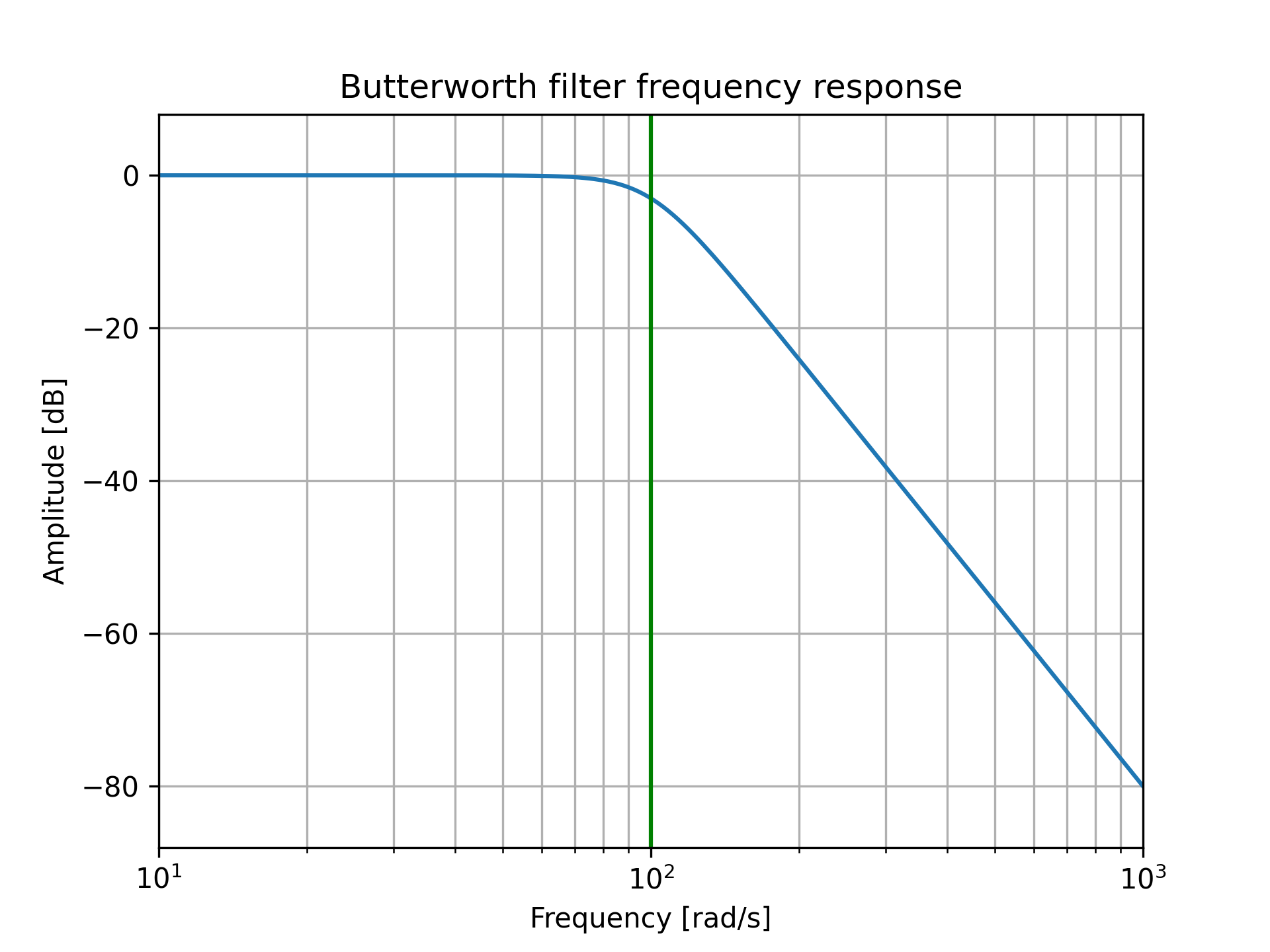
Design an analog filter and plot its frequency response, showing the critical points:from scipy import signal import matplotlib.pyplot as plt import numpy as np✓
b, a = signal.butter(4, 100, 'low', analog=True)
w, h = signal.freqs(b, a)
✓
plt.semilogx(w, 20 * np.log10(abs(h)))
plt.title('Butterworth filter frequency response')
plt.xlabel('Frequency [rad/s]')
plt.ylabel('Amplitude [dB]')
✗
plt.margins(0, 0.1)
plt.grid(which='both', axis='both')
✓
plt.axvline(100, color='green') # cutoff frequency
✗plt.show()
✓
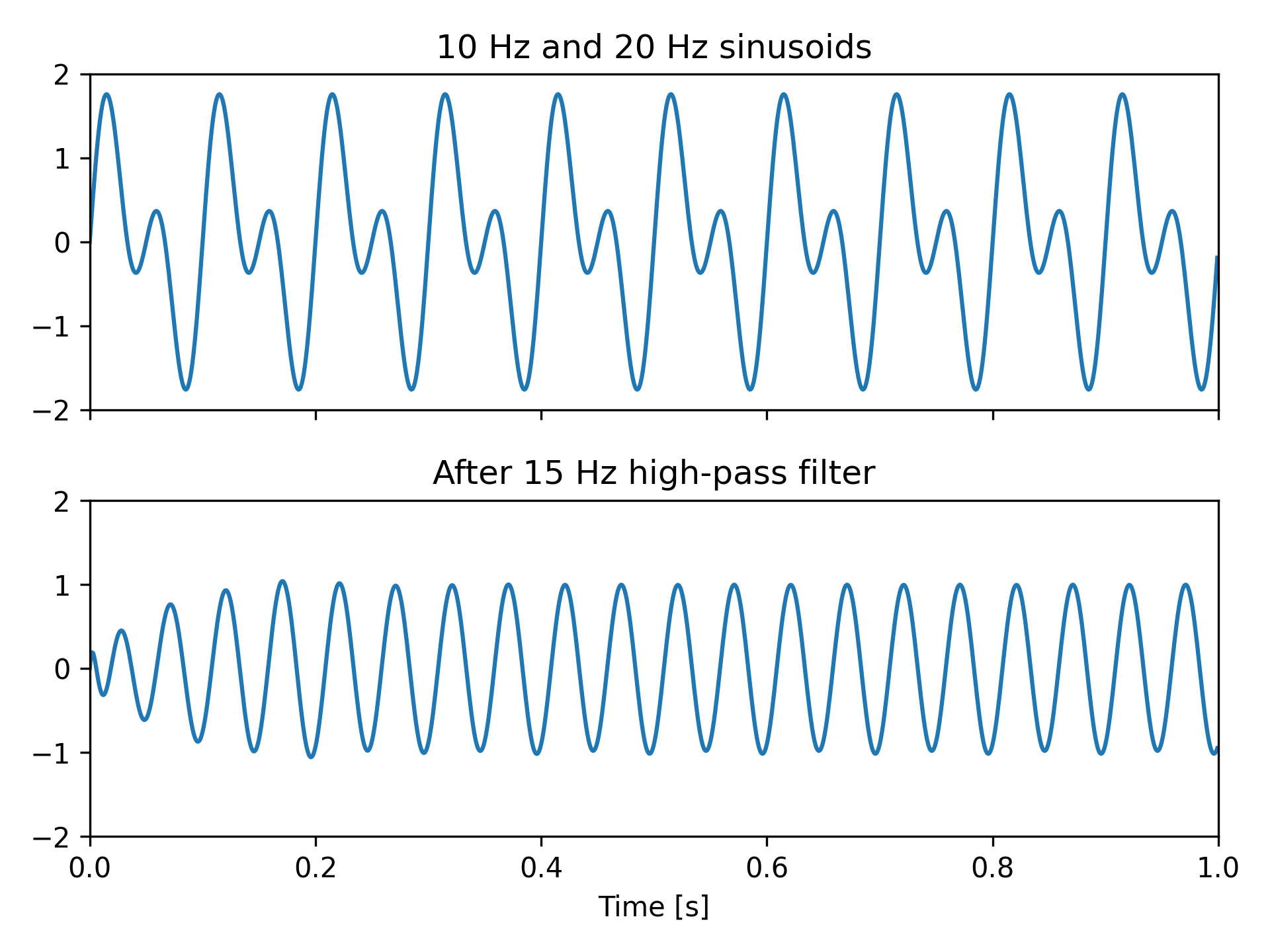
t = np.linspace(0, 1, 1000, False)  # 1 second
sig = np.sin(2*np.pi*10*t) + np.sin(2*np.pi*20*t)
fig, (ax1, ax2) = plt.subplots(2, 1, sharex=True)
✓
ax1.plot(t, sig)
ax1.set_title('10 Hz and 20 Hz sinusoids')
ax1.axis([0, 1, -2, 2])
✗
sos = signal.butter(10, 15, 'hp', fs=1000, output='sos')
filtered = signal.sosfilt(sos, sig)
✓
ax2.plot(t, filtered)
ax2.set_title('After 15 Hz high-pass filter')
ax2.axis([0, 1, -2, 2])
ax2.set_xlabel('Time [s]')
✗
plt.tight_layout()
plt.show()
✓
See also
Aliases
-
scipy.signal.butter