bundles / scipy latest / scipy / signal / _filter_design / freqz
function
scipy.signal._filter_design:freqz
Signature
def freqz ( b , a = 1 , worN = 512 , whole = False , plot = None , fs = 6.283185307179586 , include_nyquist = False ) Summary
Compute the frequency response of a digital filter.
Extended Summary
Given the M-order numerator b and N-order denominator a of a digital filter, compute its frequency response
            jw                 -jw              -jwM
   jw    B(e  )    b[0] + b[1]e    + ... + b[M]e
H(e  ) = ------ = -----------------------------------
            jw                 -jw              -jwN
         A(e  )    a[0] + a[1]e    + ... + a[N]e
Parameters
b: array_likeNumerator of a linear filter. If
bhas dimension greater than 1, it is assumed that the coefficients are stored in the first dimension, andb.shape[1:],a.shape[1:], and the shape of the frequencies array must be compatible for broadcasting.a: array_likeDenominator of a linear filter. If
bhas dimension greater than 1, it is assumed that the coefficients are stored in the first dimension, andb.shape[1:],a.shape[1:], and the shape of the frequencies array must be compatible for broadcasting.worN: {None, int, array_like}, optionalIf a single integer, then compute at that many frequencies (default is N=512). This is a convenient alternative to
np.linspace(0, fs if whole else fs/2, N, endpoint=include_nyquist)Using a number that is fast for FFT computations can result in faster computations (see Notes).
If an array_like, compute the response at the frequencies given. These are in the same units as
fs.whole: bool, optionalNormally, frequencies are computed from 0 to the Nyquist frequency, fs/2 (upper-half of unit-circle). If
wholeis True, compute frequencies from 0 to fs. Ignored if worN is array_like.plot: callableA callable that takes two arguments. If given, the return parameters w and h are passed to plot. Useful for plotting the frequency response inside freqz.
fs: float, optionalThe sampling frequency of the digital system. Defaults to 2*pi radians/sample (so w is from 0 to pi).
include_nyquist: bool, optionalIf
wholeis False andworNis an integer, settinginclude_nyquistto True will include the last frequency (Nyquist frequency) and is otherwise ignored.
Returns
w: ndarrayThe frequencies at which h was computed, in the same units as
fs. By default, w is normalized to the range [0, pi) (radians/sample).h: ndarrayThe frequency response, as complex numbers.
Notes
Using Matplotlib's matplotlib.pyplot.plot function as the callable for plot produces unexpected results, as this plots the real part of the complex transfer function, not the magnitude. Try lambda w, h: plot(w, np.abs(h)).
A direct computation via (R)FFT is used to compute the frequency response when the following conditions are met:
An integer value is given for
worN.worNis fast to compute via FFT (i.e.,next_fast_len(worN) <scipy.fft.next_fast_len>equalsworN).The denominator coefficients are a single value (
a.shape[0] == 1).worNis at least as long as the numerator coefficients (worN >= b.shape[0]).If
b.ndim > 1, thenb.shape[-1] == 1.
For long FIR filters, the FFT approach can have lower error and be much faster than the equivalent direct polynomial calculation.
Array API Standard Support
freqz has experimental support for Python Array API Standard compatible backends in addition to NumPy. Please consider testing these features by setting an environment variable SCIPY_ARRAY_API=1 and providing CuPy, PyTorch, JAX, or Dask arrays as array arguments. The following combinations of backend and device (or other capability) are supported.
====================  ====================  ====================
Library               CPU                   GPU
====================  ====================  ====================
NumPy                 ✅                     n/a
CuPy                  n/a                   ✅
PyTorch               ✅                     ✅
JAX                   ⚠️ no JIT             ⛔
Dask                  ⚠️ computes graph     n/a
====================  ====================  ====================
See
dev-arrayapifor more information.
Examples
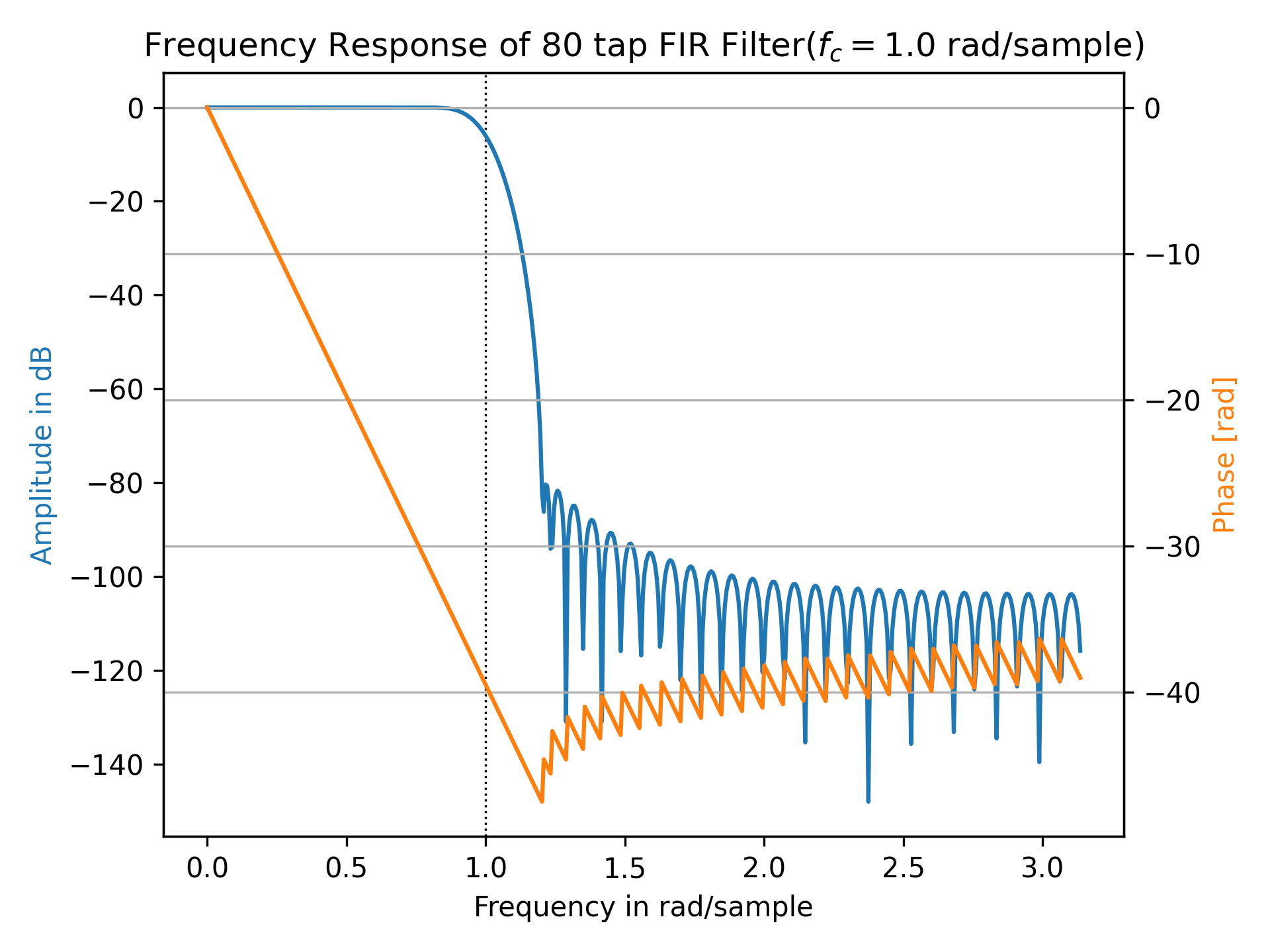
from scipy import signal
import numpy as np
taps, f_c = 80, 1.0  # number of taps and cut-off frequency
b = signal.firwin(taps, f_c, window=('kaiser', 8), fs=2*np.pi)
w, h = signal.freqz(b)
✓
import matplotlib.pyplot as plt
fig, ax1 = plt.subplots(tight_layout=True)
✓
ax1.set_title(f"Frequency Response of {taps} tap FIR Filter" +
              f"($f_c={f_c}$ rad/sample)")
ax1.axvline(f_c, color='black', linestyle=':', linewidth=0.8)
ax1.plot(w, 20 * np.log10(abs(h)), 'C0')
ax1.set_ylabel("Amplitude in dB", color='C0')
ax1.set(xlabel="Frequency in rad/sample", xlim=(0, np.pi))
✗
ax2 = ax1.twinx()
phase = np.unwrap(np.angle(h))
✓
ax2.plot(w, phase, 'C1')
ax2.set_ylabel('Phase [rad]', color='C1')
✗
ax2.grid(True)
✓ax2.axis('tight')
✗plt.show()
✓
rng = np.random.default_rng()
b = rng.random((2, 25))
✓
w, h = signal.freqz(b.T[..., np.newaxis], worN=1024)
w.shape
h.shape
✓
b = np.array([0.5, 0.5])
a = np.array([[1, 1], [-0.25, -0.5]])
✓
w, h = signal.freqz(b, a[..., np.newaxis], worN=1024)
w.shape
h.shape
✓
See also
Aliases
-
scipy.signal.freqz