bundles / scipy latest / scipy / signal / _filter_design / freqz_sos
function
scipy.signal._filter_design:freqz_sos
Signature
def freqz_sos ( sos , worN = 512 , whole = False , fs = 6.283185307179586 ) Summary
Compute the frequency response of a digital filter in SOS format.
Extended Summary
Given sos, an array with shape (n, 6) of second order sections of a digital filter, compute the frequency response of the system function
       B0(z)   B1(z)         B{n-1}(z)
H(z) = ----- * ----- * ... * ---------
       A0(z)   A1(z)         A{n-1}(z)
for z = exp(omega*1j), where B{k}(z) and A{k}(z) are numerator and denominator of the transfer function of the k-th second order section.
Parameters
sos: array_likeArray of second-order filter coefficients, must have shape
(n_sections, 6). Each row corresponds to a second-order section, with the first three columns providing the numerator coefficients and the last three providing the denominator coefficients.worN: {None, int, array_like}, optionalIf a single integer, then compute at that many frequencies (default is N=512). Using a number that is fast for FFT computations can result in faster computations (see Notes of freqz).
If an array_like, compute the response at the frequencies given (must be 1-D). These are in the same units as
fs.whole: bool, optionalNormally, frequencies are computed from 0 to the Nyquist frequency, fs/2 (upper-half of unit-circle). If
wholeis True, compute frequencies from 0 to fs.fs: float, optionalThe sampling frequency of the digital system. Defaults to 2*pi radians/sample (so w is from 0 to pi).
Returns
w: ndarrayThe frequencies at which h was computed, in the same units as
fs. By default, w is normalized to the range [0, pi) (radians/sample).h: ndarrayThe frequency response, as complex numbers.
Notes
This function used to be called sosfreqz in older versions (≥ 0.19.0)
Array API Standard Support
freqz_sos has experimental support for Python Array API Standard compatible backends in addition to NumPy. Please consider testing these features by setting an environment variable SCIPY_ARRAY_API=1 and providing CuPy, PyTorch, JAX, or Dask arrays as array arguments. The following combinations of backend and device (or other capability) are supported.
====================  ====================  ====================
Library               CPU                   GPU
====================  ====================  ====================
NumPy                 ✅                     n/a
CuPy                  n/a                   ✅
PyTorch               ✅                     ✅
JAX                   ⚠️ no JIT             ⛔
Dask                  ⚠️ computes graph     n/a
====================  ====================  ====================
See
dev-arrayapifor more information.
Examples
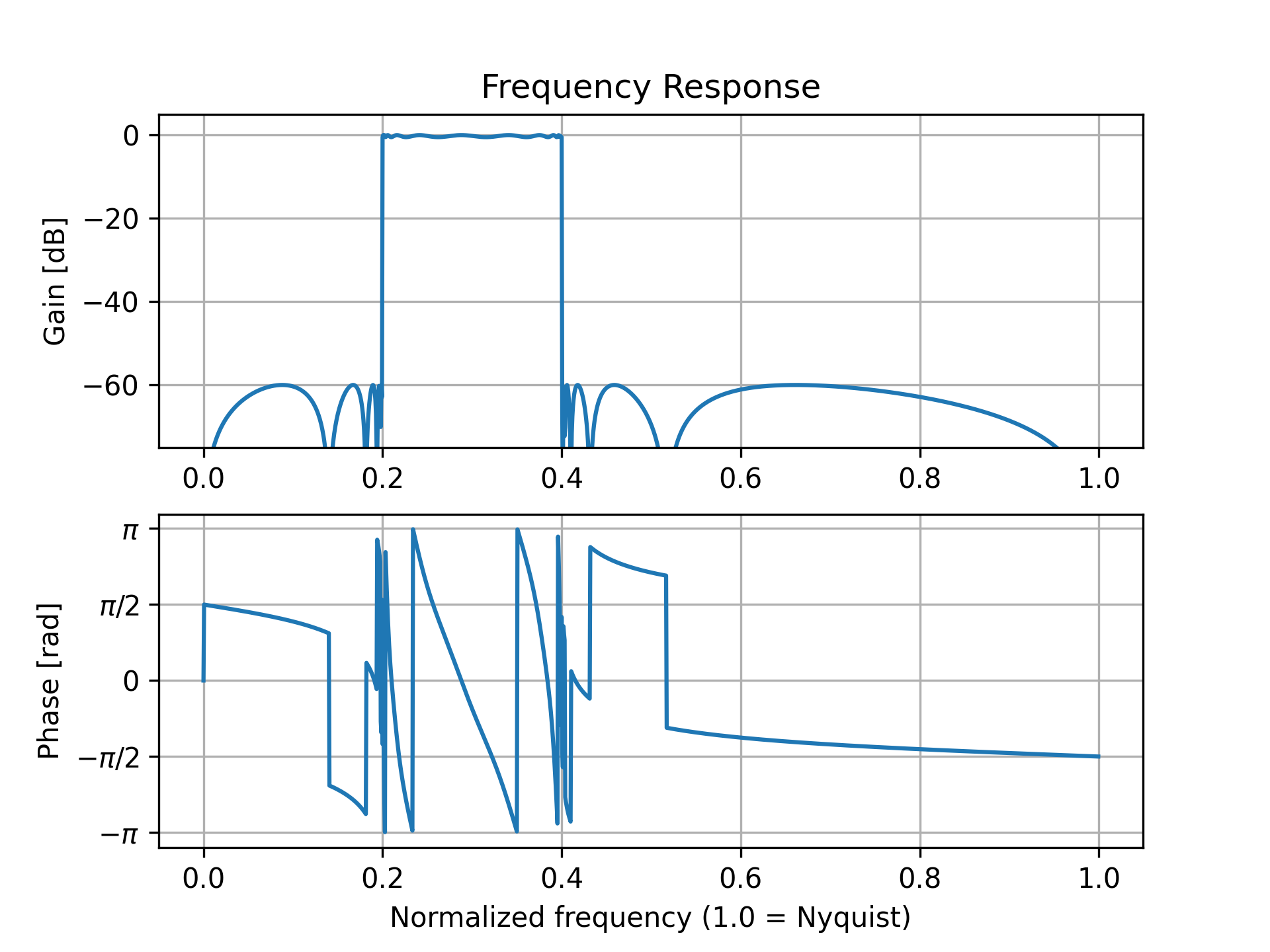
Design a 15th-order bandpass filter in SOS format.from scipy import signal import numpy as np sos = signal.ellip(15, 0.5, 60, (0.2, 0.4), btype='bandpass', output='sos')✓
w, h = signal.freqz_sos(sos, worN=1500)
✓import matplotlib.pyplot as plt
✓plt.subplot(2, 1, 1)
✗db = 20*np.log10(np.maximum(np.abs(h), 1e-5))
✓plt.plot(w/np.pi, db) plt.ylim(-75, 5)✗
plt.grid(True)
✓plt.yticks([0, -20, -40, -60]) plt.ylabel('Gain [dB]') plt.title('Frequency Response') plt.subplot(2, 1, 2) plt.plot(w/np.pi, np.angle(h))✗
plt.grid(True)
✓plt.yticks([-np.pi, -0.5*np.pi, 0, 0.5*np.pi, np.pi], [r'$-\pi$', r'$-\pi/2$', '0', r'$\pi/2$', r'$\pi$']) plt.ylabel('Phase [rad]') plt.xlabel('Normalized frequency (1.0 = Nyquist)')✗
plt.show()
✓
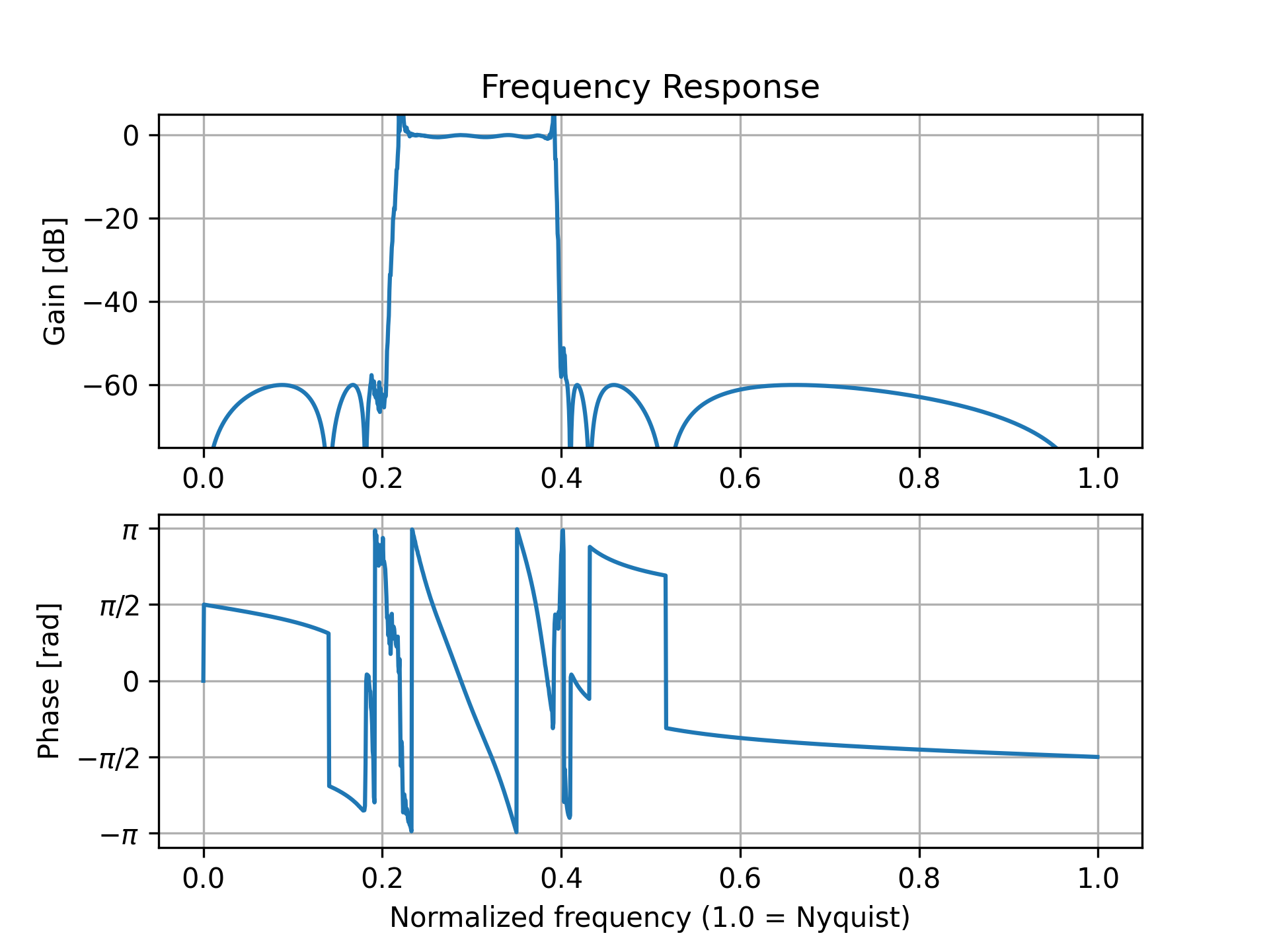
b, a = signal.ellip(15, 0.5, 60, (0.2, 0.4), btype='bandpass',
                   output='ba')
w, h = signal.freqz(b, a, worN=1500)
✓
plt.subplot(2, 1, 1)
✗db = 20*np.log10(np.maximum(np.abs(h), 1e-5))
✓plt.plot(w/np.pi, db) plt.ylim(-75, 5)✗
plt.grid(True)
✓plt.yticks([0, -20, -40, -60]) plt.ylabel('Gain [dB]') plt.title('Frequency Response') plt.subplot(2, 1, 2) plt.plot(w/np.pi, np.angle(h))✗
plt.grid(True)
✓plt.yticks([-np.pi, -0.5*np.pi, 0, 0.5*np.pi, np.pi], [r'$-\pi$', r'$-\pi/2$', '0', r'$\pi/2$', r'$\pi$']) plt.ylabel('Phase [rad]') plt.xlabel('Normalized frequency (1.0 = Nyquist)')✗
plt.show()
✓
See also
Aliases
-
scipy.signal.freqz_sos