`scipy.signal._signaltools:hilbert`

source: /scipy/signal/_signaltools.py :2410

Signature

def hilbert ( x , N = None , axis = -1 )

Summary

FFT-based computation of the analytic signal.

Extended Summary

The analytic signal is calculated by zeroing out the negative frequencies and doubling the amplitudes of the positive frequencies in the FFT domain. The imaginary part of the result is the hilbert transform of the real-valued input signal.

The transformation is done along the last axis by default.

For numpy arrays, scipy.fft.set_workers can be used to change the number of workers used for the FFTs.

Parameters

x : array_like: Signal data. Must be real.
N : int, optional: Number of output samples. x is initially cropped or zero-padded to length N along axis. Default: x.shape[axis]
axis : int, optional: Axis along which to do the transformation. Default: -1.

Returns

xa : ndarray: Analytic signal of x, of each 1-D array along axis

Notes

The analytic signal x_a(t) of a real-valued signal x(t) can be expressed as ^[1]

x_{a} = F^{- 1} (F (x) 2 U) = x + i y,

where F is the Fourier transform, U the unit step function, and y the Hilbert transform of x. ^[2]

In other words, the negative half of the frequency spectrum is zeroed out, turning the real-valued signal into a complex-valued signal. The Hilbert transformed signal can be obtained from np.imag(hilbert(x)), and the original signal from np.real(hilbert(x)).

Array API Standard Support

hilbert has experimental support for Python Array API Standard compatible backends in addition to NumPy. Please consider testing these features by setting an environment variable SCIPY_ARRAY_API=1 and providing CuPy, PyTorch, JAX, or Dask arrays as array arguments. The following combinations of backend and device (or other capability) are supported.

====================  ====================  ====================
Library               CPU                   GPU
====================  ====================  ====================
NumPy                 ✅                     n/a                 
CuPy                  n/a                   ✅                   
PyTorch               ✅                     ✅                   
JAX                   ⛔                     ⛔                   
Dask                  ✅                     n/a                 
====================  ====================  ====================

See dev-arrayapi for more information.

Examples

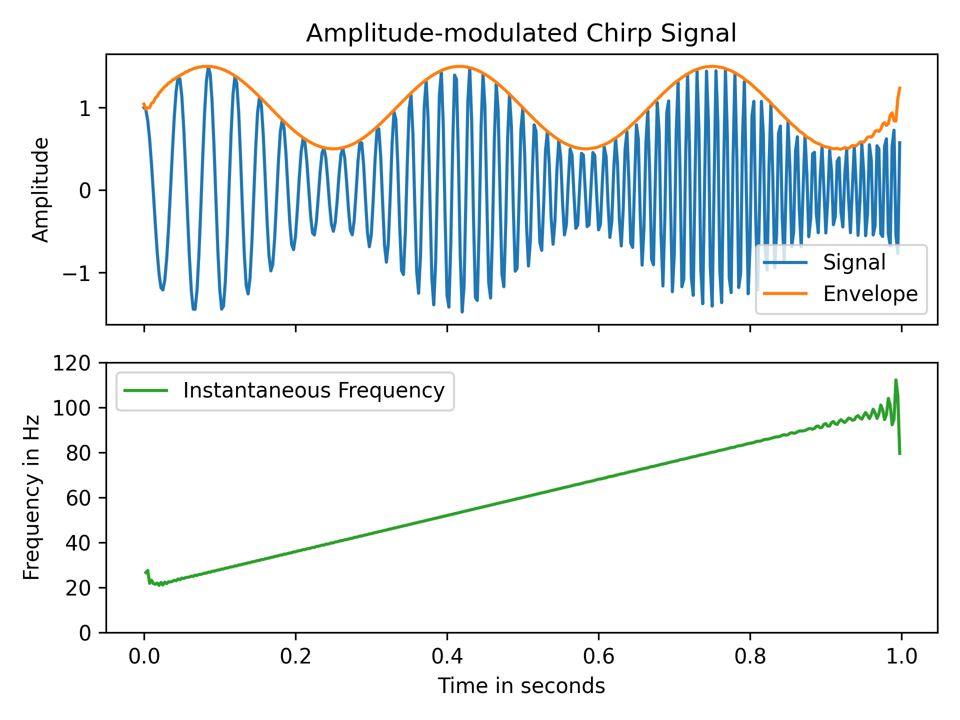
In this example we use the Hilbert transform to determine the amplitude envelope and instantaneous frequency of an amplitude-modulated signal. Let's create a chirp of which the frequency increases from 20 Hz to 100 Hz and apply an amplitude modulation:

import numpy as np
import matplotlib.pyplot as plt
from scipy.signal import hilbert, chirp
duration, fs = 1, 400  # 1 s signal with sampling frequency of 400 Hz
t = np.arange(int(fs*duration)) / fs  # timestamps of samples
signal = chirp(t, 20.0, t[-1], 100.0)
signal *= (1.0 + 0.5 * np.sin(2.0*np.pi*3.0*t) )

✓

The amplitude envelope is given by the magnitude of the analytic signal. The instantaneous frequency can be obtained by differentiating the instantaneous phase in respect to time. The instantaneous phase corresponds to the phase angle of the analytic signal.

analytic_signal = hilbert(signal)
amplitude_envelope = np.abs(analytic_signal)
instantaneous_phase = np.unwrap(np.angle(analytic_signal))
instantaneous_frequency = np.diff(instantaneous_phase) / (2.0*np.pi) * fs
fig, (ax0, ax1) = plt.subplots(nrows=2, sharex='all', tight_layout=True)

✓

ax0.set_title("Amplitude-modulated Chirp Signal")
ax0.set_ylabel("Amplitude")
ax0.plot(t, signal, label='Signal')
ax0.plot(t, amplitude_envelope, label='Envelope')
ax0.legend()
ax1.set(xlabel="Time in seconds", ylabel="Frequency in Hz", ylim=(0, 120))
ax1.plot(t[1:], instantaneous_frequency, 'C2-',
         label='Instantaneous Frequency')
ax1.legend()

✗

plt.show()

✓

Aliases

scipy.signal.hilbert