bundles / scipy latest / scipy / signal / _signaltools / resample
function
scipy.signal._signaltools:resample
Signature
def resample ( x , num , t = None , axis = 0 , window = None , domain = time ) Summary
Resample x to num samples using the Fourier method along the given axis.
Extended Summary
The resampling is performed by shortening or zero-padding the FFT of x. This has the advantages of providing an ideal antialiasing filter and allowing arbitrary up- or down-sampling ratios. The main drawback is the requirement of assuming x to be a periodic signal.
Parameters
x: array_likeThe input signal made up of equidistant samples. If
xis a multidimensional array, the parameteraxisspecifies the time/frequency axis. It is assumed here thatn_x = x.shape[axis]specifies the number of samples andTthe sampling interval.num: intThe number of samples of the resampled output signal. It may be larger or smaller than
n_x.t: array_like, optionalIf
tis notNone, then the timestamps of the resampled signal are also returned.tmust contain at least the first two timestamps of the input signalx(all others are ignored). The timestamps of the output signal are determined byt[0] + T * n_x / num * np.arange(num)withT = t[1] - t[0]. Default isNone.axis: int, optionalThe time/frequency axis of
xalong which the resampling take place. The Default is 0.window: array_like, callable, string, float, or tuple, optionalIf not
None, it specifies a filter in the Fourier domain, which is applied before resampling. I.e., the FFTXofxis calculated byX = W * fft(x, axis=axis).Wmay be interpreted as a spectral windowing functionW(f_X)which consumes the frequenciesf_X = fftfreq(n_x, T).If
windowis a 1d array of lengthn_xthenW=window. Ifwindowis a callable thenW = window(f_X). Otherwise,windowis passed to get_window, i.e.,W = fftshift(signal.get_window(window, n_x)). Default isNone.domain: 'time' | 'freq', optionalIf set to
'time'(default) then an FFT is applied tox, otherwise ('freq') it is asssmued that an FFT was already applied, i.e.,x = fft(x_t, axis=axis)withx_tbeing the input signal in the time domain.
Returns
x_r: ndarrayThe resampled signal made up of
numsamples and sampling intervalT * n_x / num.t_r: ndarray, optionalThe
numequidistant timestamps of x_r. This is only returned if paramatertis notNone.
Notes
This function uses the more efficient one-sided FFT, i.e. rfft / irfft, if x is real-valued and in the time domain. Else, the two-sided FFT, i.e., fft / ifft, is used (all FFT functions are taken from the scipy.fft module).
If a window is applied to a real-valued x, the one-sided spectral windowing function is determined by taking the average of the negative and the positive frequency component. This ensures that real-valued signals and complex signals with zero imaginary part are treated identically. I.e., passing x or passing x.astype(np.complex128) produce the same numeric result.
If the number of input or output samples are prime or have few prime factors, this function may be slow due to utilizing FFTs. Consult prev_fast_len and next_fast_len for determining efficient signals lengths. Alternatively, utilizing resample_poly to calculate an intermediate signal (as illustrated in the example below) can result in significant speed increases.
resample is intended to be used for periodic signals with equidistant sampling intervals. For non-periodic signals, resample_poly may be a better choice. Consult the scipy.interpolate module for methods of resampling signals with non-constant sampling intervals.
Array API Standard Support
resample has experimental support for Python Array API Standard compatible backends in addition to NumPy. Please consider testing these features by setting an environment variable SCIPY_ARRAY_API=1 and providing CuPy, PyTorch, JAX, or Dask arrays as array arguments. The following combinations of backend and device (or other capability) are supported.
====================  ====================  ====================
Library               CPU                   GPU
====================  ====================  ====================
NumPy                 ✅                     n/a
CuPy                  n/a                   ✅
PyTorch               ✅                     ⛔
JAX                   ⛔                     ⛔
Dask                  ⛔                     n/a
====================  ====================  ====================
See
dev-arrayapifor more information.
Examples
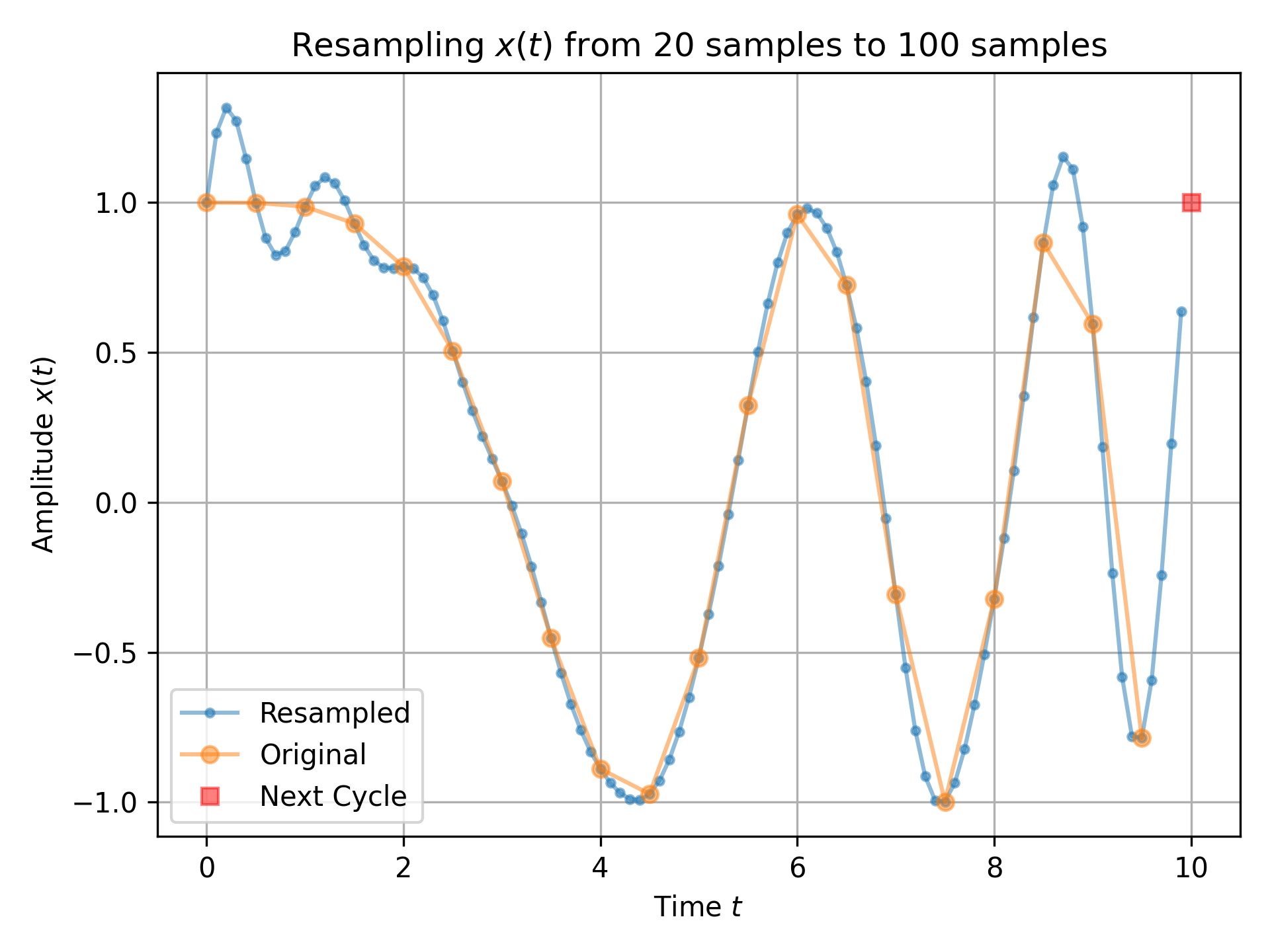
The following example depicts a signal being up-sampled from 20 samples to 100 samples. The ringing at the beginning of the up-sampled signal is due to interpreting the signal being periodic. The red square in the plot illustrates that periodictiy by showing the first sample of the next cycle of the signal.import numpy as np import matplotlib.pyplot as plt from scipy.signal import resample n0, n1 = 20, 100 # number of samples t0 = np.linspace(0, 10, n0, endpoint=False) # input time stamps x0 = np.cos(-t0**2/6) # input signal x1 = resample(x0, n1) # resampled signal t1 = np.linspace(0, 10, n1, endpoint=False) # timestamps of x1 fig0, ax0 = plt.subplots(1, 1, tight_layout=True)✓
ax0.set_title(f"Resampling $x(t)$ from {n0} samples to {n1} samples")
ax0.set(xlabel="Time $t$", ylabel="Amplitude $x(t)$")
ax0.plot(t1, x1, '.-', alpha=.5, label=f"Resampled")
ax0.plot(t0, x0, 'o-', alpha=.5, label="Original")
ax0.plot(10, x0[0], 'rs', alpha=.5, label="Next Cycle")
ax0.legend(loc='best')
✗
ax0.grid(True)
plt.show()
✓
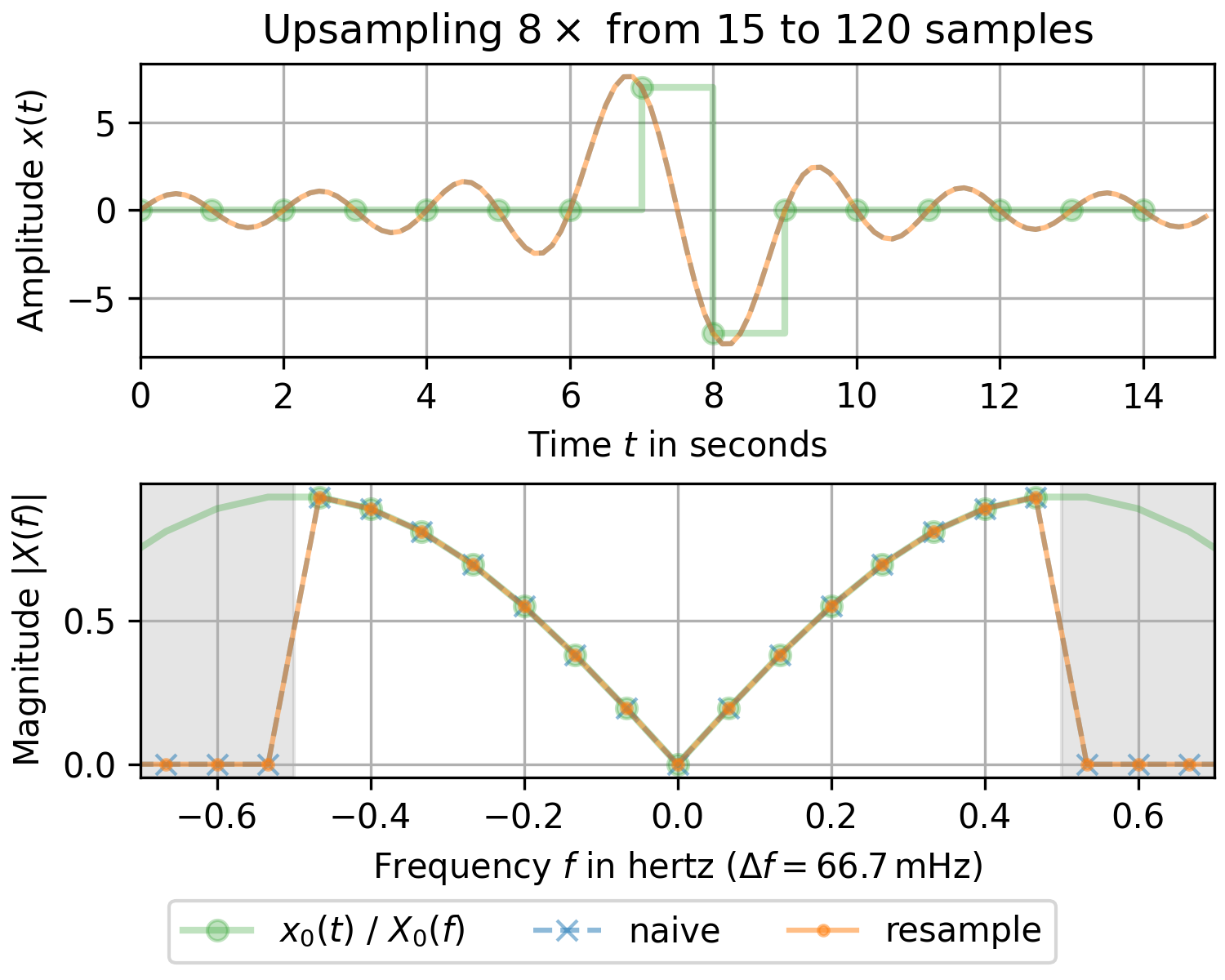
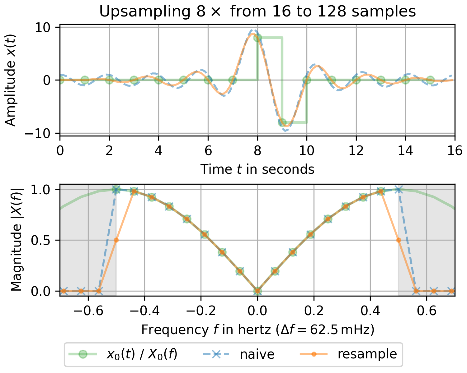
import matplotlib.pyplot as plt
import numpy as np
from scipy.fft import fftshift, fftfreq, fft, rfft, irfft
from scipy.signal import resample, resample_poly
fac, T0, T1 = 8, 1, 1/8  # upsampling factor and sampling intervals
✓
for n0 in (15, 16):  # number of samples of input signal
    n1 = fac * n0  # number of samples of upsampled signal
    t0, t1 = T0 * np.arange(n0), T1 * np.arange(n1)  # time stamps
    x0 = np.zeros(n0)  # input signal has two non-zero sample values
    x0[n0//2], x0[n0//2+1] = n0 // 2, -(n0 // 2)

    x1n = irfft(rfft(x0), n=n1) * n1 / n0  # naive resampling
    x1r = resample(x0, n1)  # resample signal

    # Determine magnitude spectrum:
    x0_up = np.zeros_like(x1r)  # upsampling without antialiasing filter
    x0_up[::n1 // n0] = x0
    X0, X0_up = (fftshift(fft(x_)) / n0 for x_ in (x0, x0_up))
    XX1 = (fftshift(fft(x_)) / n1 for x_ in (x1n, x1r))
    f0, f1 = fftshift(fftfreq(n0, T0)), fftshift(fftfreq(n1, T1))  # frequencies
    df = f0[1] - f0[0]  # frequency resolution

    fig, (ax0, ax1) = plt.subplots(2, 1, layout='constrained', figsize=(5, 4))
    ax0.set_title(rf"Upsampling ${fac}\times$ from {n0} to {n1} samples")
    ax0.set(xlabel="Time $t$ in seconds", ylabel="Amplitude $x(t)$",
            xlim=(0, n1*T1))
    ax0.step(t0, x0, 'C2o-', where='post', alpha=.3, linewidth=2,
             label="$x_0(t)$ / $X_0(f)$")
    for x_, l_ in zip((x1n, x1r), ('C0--', 'C1-')):
        ax0.plot(t1, x_, l_, alpha=.5, label=None)
    ax0.grid()
    ax1.set(xlabel=rf"Frequency $f$ in hertz ($\Delta f = {df*1e3:.1f}\,$mHz)",
            ylabel="Magnitude $|X(f)|$", xlim=(-0.7, 0.7))
    ax1.axvspan(0.5/T0, f1[-1], color='gray', alpha=.2)
    ax1.axvspan(f1[0], -0.5/T0, color='gray', alpha=.2)
    ax1.plot(f1, abs(X0_up), 'C2-', f0, abs(X0),  'C2o', alpha=.3, linewidth=2)
    for X_, n_, l_ in zip(XX1, ("naive", "resample"), ('C0x--', 'C1.-')):
        ax1.plot(f1, abs(X_), l_, alpha=.5, label=n_)
    ax1.grid()
    fig.legend(loc='outside lower center', ncols=4)
✗
plt.show()
✓
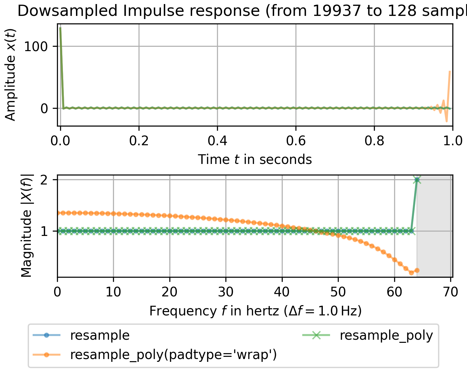
import matplotlib.pyplot as plt
import numpy as np
from scipy.fft import rfftfreq, rfft
from scipy.signal import resample, resample_poly
n0 = 19937 # number of input samples - prime
n1 = 128  # number of output samples - fast FFT length
T0, T1 = 1/n0, 1/n1  # sampling intervals
t0, t1 = np.arange(n0)*T0, np.arange(n1)*T1  # time stamps
x0 = np.zeros(n0)  # Input has one non-zero sample
x0[0] = n0
x1r = resample(x0, n1)  # slow due to n0 being prime
x1p = resample(resample_poly(x0, 1, n0 // n1, padtype='wrap'), n1)  # periodic
x2p = resample(resample_poly(x0, 1, n0 // n1), n1)  # with zero-padding
X0 = rfft(x0) / n0
X1r, X1p, X2p = rfft(x1r) / n1, rfft(x1p) / n1, rfft(x2p) / n1
f0, f1 = rfftfreq(n0, T0), rfftfreq(n1, T1)
fig, (ax0, ax1) = plt.subplots(2, 1, layout='constrained', figsize=(5, 4))
✓
ax0.set_title(f"Dowsampled Impulse response (from {n0} to {n1} samples)")
ax0.set(xlabel="Time $t$ in seconds", ylabel="Amplitude $x(t)$", xlim=(-T1, 1))
for x_ in (x1r, x1p, x2p):
    ax0.plot(t1, x_, alpha=.5)
✗
ax0.grid()
✓ax1.set(xlabel=rf"Frequency $f$ in hertz ($\Delta f = {f1[1]}\,$Hz)", ylabel="Magnitude $|X(f)|$", xlim=(0, 0.55/T1)) ax1.axvspan(0.5/T1, f0[-1], color='gray', alpha=.2) ax1.plot(f1, abs(X1r), 'C0.-', alpha=.5, label="resample") ax1.plot(f1, abs(X1p), 'C1.-', alpha=.5, label="resample_poly(padtype='wrap')") ax1.plot(f1, abs(X2p), 'C2x-', alpha=.5, label="resample_poly")✗
ax1.grid()
✓fig.legend(loc='outside lower center', ncols=2)
✗plt.show()
✓
See also
- decimate
Downsample a (periodic/non-periodic) signal after applying an FIR or IIR filter.
- resample_poly
Resample a (periodic/non-periodic) signal using polyphase filtering and an FIR filter.
Aliases
-
scipy.signal.resample